生物信息与R语言QQ群: 187923577
Tips: 看不清代码请刷新,换个颜色再看。
1. 比较干净的背景: +theme_bw(); 最干净的背景: +theme_classic()
2. 参数的解释: 生物慕课网
3. 本页面最底部有生信QQ群号,欢迎加入讨论,严禁广告。
#############################
library(ggplot2)
library(reshape2)
#示例数据:某基因在对照和肿瘤样本中的表达量。
d1=data.frame(
control=c(10,20,30,40,30,60,20,40,20,20,10,20,30,40,30,40,20,40,20,20),
tumor=c(50,70,40,60,80,90,40,50,70,80,50,70,40,60,80,90,40,50,70,80)
);
# 数据框重塑,数据合并为一列,添加分类列
d2=melt(d1,
variable.name="type",#新变量的名字
value.name="value" #值得名字
);
d2
######## 开始画图1 箱线图 + 散点图 done
ggplot(d2,aes(factor(type), value))+
geom_boxplot()+
geom_jitter()
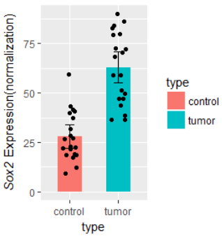
######## 开始画图2 带误差bar的柱状图 + 散点图 done
#http://www.cookbook-r.com/Manipulating_data/Summarizing_data/
## Summarizes data.
## Gives count, mean, standard deviation, standard error of the mean, and confidence interval (default 95%).
## data: a data frame.
## measurevar: the name of a column that contains the variable to be summariezed
## groupvars: a vector containing names of columns that contain grouping variables
## na.rm: a boolean that indicates whether to ignore NA's
## conf.interval: the percent range of the confidence interval (default is 95%)
summarySE = function(data=NULL, measurevar, groupvars=NULL, na.rm=FALSE,
conf.interval=.95, .drop=TRUE) {
library(plyr)
# New version of length which can handle NA's: if na.rm==T, don't count them
length2 = function (x, na.rm=FALSE) {
if (na.rm) sum(!is.na(x))
else length(x)
}
# This does the summary. For each group's data frame, return a vector with
# N, mean, and sd
datac = ddply(data, groupvars, .drop=.drop,
.fun = function(xx, col) {
c(N = length2(xx[[col]], na.rm=na.rm),
mean = mean (xx[[col]], na.rm=na.rm),
sd = sd (xx[[col]], na.rm=na.rm)
)
},
measurevar
)
# Rename the "mean" column
datac = rename(datac, c("mean" = measurevar))
datac$se = datac$sd / sqrt(datac$N) # Calculate standard error of the mean
# Confidence interval multiplier for standard error
# Calculate t-statistic for confidence interval:
# e.g., if conf.interval is .95, use .975 (above/below), and use df=N-1
ciMult = qt(conf.interval/2 + .5, datac$N-1)
datac$ci = datac$se * ciMult
return(datac)
}
# http://www.cookbook-r.com/Graphs/Plotting_means_and_error_bars_(ggplot2)/
d3 = summarySE(d2, measurevar="value", groupvars=c("type"))
d3
ggplot(d3, aes(x=type, y=value)) +
geom_bar(aes(fill=type),position=position_dodge(), stat="identity", width=0.5) +
geom_errorbar(aes(ymin=value-ci, ymax=value+ci),
width=.2, # Width of the error bars
position=position_dodge(.9))+
geom_jitter(data=d2,aes(type,value), width=0.15) +
ylab( expression(paste( italic("Sox2")," Expression(normalization)") ) )
#ylab("Sox2 Expression\n(normalization)")
小遗憾: 不能把bar和x轴之间的距离去掉;使用 scale_y_continuous( #expand = c(0,0)) 会导致顶部的 显著性星号不显示。
todo: 批量bar图,一次显示多个基因的差异。
counts_dir="/home/wangjl/data/rsa/kasumi-1/"

# 载入 summarySE 函数,见上文 1 中的代码。

# 1.load data----
kasumi.raw=read.table("/home/wangjl/data/rsa/kasumi-1/counts/featureCounts_SRR1124_matrix2.txt",
           skip = 1, row.names = 1, header = T)

gene.counts = kasumi.raw[, 6:ncol(kasumi.raw)] #col5 length
colnames(gene.counts) = sub("map.", "", colnames(gene.counts))
colnames(gene.counts) = sub("_Aligned.sortedByCoord.out.bam", "", colnames(gene.counts))
colnames(gene.counts)|>jsonlite::toJSON()
# ["SRR11247521","SRR11247522","SRR11247523","SRR11247524", wt
#  "SRR11247525","SRR11247526","SRR11247527","SRR11247528", kd1
#  "SRR11247529","SRR11247530","SRR11247531","SRR11247532"] kd2

gene.counts[1:5, 1:2]

# rm all 0 rows
dim(gene.counts) #61209    12
gene.counts = gene.counts[ rowSums(gene.counts)>0, ]
dim(gene.counts) #35330    12

gene.counts[1:5, 1:10]

gene.length = kasumi.raw[rownames(gene.counts),'Length']


#2. normalize to TPM ----
gene.tpm=apply(gene.counts, 2, function(x){
  x1=x/gene.length
  x1/sum(x1)*1e6
})

dim(gene.tpm) #35330 个基因,12个样本


#3. draw bar plot with error bar and significance ----
gene.symbol ="ITGAM"
# get data
gene.long = data.frame(
  value = gene.tpm[gene.symbol,],
  type = c( rep("wt",4), rep('kd1', 4), rep('kd2', 4) ),
  gene=gene.symbol
)

gene.long$type=factor(gene.long$type, levels = c("wt", 'kd1', 'kd2') )
gene.long |> head()

> gene.long
                value type  gene
SRR11247521 1.4256497   wt ITGAM
SRR11247522 2.0270137   wt ITGAM
SRR11247523 0.7544062   wt ITGAM
SRR11247524 0.9217557   wt ITGAM
SRR11247525 4.0224827  kd1 ITGAM
SRR11247526 3.6449108  kd1 ITGAM
SRR11247527 3.6758330  kd1 ITGAM
SRR11247528 3.5564203  kd1 ITGAM
SRR11247529 6.8501709  kd2 ITGAM
SRR11247530 6.9693542  kd2 ITGAM
SRR11247531 7.2995709  kd2 ITGAM
SRR11247532 7.8914830  kd2 ITGAM


## mean among group ----
sapply( split(gene.long$value, gene.long$type), mean )
#      wt      kd1      kd2
#1.282206 3.724912 7.252645


## P value among group ----
#gene.long$type
> t.test(gene.long$value[1:4], gene.long$value[5:8] )$p.value #kd1 vs wt
[1] 0.001694615
> t.test(gene.long$value[1:4], gene.long$value[9:12] )$p.value #kd2 vs wt
[1] 5.068546e-06


## bar plot ----
library(ggplot2)
d2=gene.long # for jitter
d3 = summarySE(gene.long, measurevar="value", groupvars=c("type")) #画 barplot

#BiocManager::install('ggsignif')
library("ggsignif")
my_comparisons = list(c("wt","kd1"), c("wt","kd2"))

set.seed(2023)
ggplot(d3, aes(x=type, y=value)) +
  geom_bar(aes(fill=type), position=position_dodge(), stat="identity",
           width=0.8, show.legend = F) +
  geom_errorbar(aes(ymin=value-ci, ymax=value+ci), #误差棒
                width=.2, # Width of the error bars
                position=position_dodge(.9)) +
  geom_jitter(data=d2, aes(type,value), width=0.15, size=1) + #散点
  geom_signif(data=d2, comparisons = my_comparisons, #显著性 星号
              step_increase = 0.12,
              map_signif_level = T, #T显示星号,F显示p值
              test = t.test, size=0.5,textsize = 4)+
  xlab("")+
  ylab(bquote(paste( italic( .(gene.symbol) ), " Expression(TPM)") ) ) +
  #scale_y_discrete(expand = c(0,0)) +
  scale_y_continuous( #expand = c(0,0),
                     limits = c(0, max(d2$value)*1.2)) +
  scale_x_discrete( limits=c("wt", "kd1", "kd2"),
                    breaks=c("wt", "kd1", "kd2"),
                    labels=c("shControl", "shFIP1L1(1)", "shFIP1L1(2)") ) +
  theme_classic(base_size = 12) +
  theme(
    #plot.title=element_text(size = 12),
    #axis.title.x=element_text(size = 12),
    #axis.title.y=element_text(size = 12),
    axis.text.x = element_text(angle = 45, hjust = 1, colour = "black", size = 12),
    axis.text.y=element_text(size=12, color="black")
  )+
  scale_fill_manual(breaks = c("wt", "kd1", "kd2"),
                    values=c("#ed553b", "#99b433", "#00a300"))

#
ggsave( paste0("FIP1L1_KD/Kasumi-1_FIP1L1_KD_",gene.symbol,".pdf"), width =1.68, height=3.2)
批量显示多个基因的mean+-sd。
# plot iris's 4 features's bar plot with sd, by Species
dat.avg=do.call(rbind, lapply(split(iris[,1:4], iris$Species), function(x){
  colMeans(x)
}))
dat.avg
#           Sepal.Length Sepal.Width Petal.Length Petal.Width
#setosa            5.006       3.428        1.462       0.246
#versicolor        5.936       2.770        4.260       1.326
#virginica         6.588       2.974        5.552       2.026

dat.sd=do.call(rbind, lapply(split(iris[,1:4], iris$Species), function(x){
  apply(x, 2, sd)
}))
dat.sd
#           Sepal.Length Sepal.Width Petal.Length Petal.Width
#setosa        0.3524897   0.3790644    0.1736640   0.1053856
#versicolor    0.5161711   0.3137983    0.4699110   0.1977527
#virginica     0.6358796   0.3224966    0.5518947   0.2746501

# melt
dat=reshape2::melt(dat.avg)
colnames(dat)=c("type", "feature", "avg")
dat$sd=reshape2::melt(dat.sd)$value
head(dat, 3)
#        type      feature   avg        sd
#1     setosa Sepal.Length 5.006 0.3524897
#2 versicolor Sepal.Length 5.936 0.5161711
#3  virginica Sepal.Length 6.588 0.6358796

pdf(paste0(outputRoot, "xx_barplot-with-error-bar.pdf"), width=4, height = 2.6)
ggplot(dat) +
  geom_bar( aes(x=type, y=avg, fill=type), stat="identity", alpha=0.7, show.legend = F) +
  geom_errorbar( aes(x=type, ymin=avg-sd, ymax=avg+sd),
                 width=0.3, colour="black", alpha=1, size=0.5)+
  facet_grid(~feature)+
  scale_fill_manual(values = c("#fde725",  "#3ac96d",  "#440154"))+
  theme_classic(base_size = 12)+
  theme(
    axis.text.x = element_text(angle = 45, hjust = 1, size = 12),
    strip.background = element_blank(), #top strip border
    strip.text = element_text(size = 10, face = "italic")
  )+
  labs(x="", y="Average Value")
dev.off()


if(0){
  #https://r-graph-gallery.com/4-barplot-with-error-bar.html
  #sd
  sd <- sd(vec)
  sd <- sqrt(var(vec))
  #se
  se = sd(vec) / sqrt(length(vec))
  # ci
  alpha=0.05
  t=qt((1-alpha)/2 + .5, length(vec)-1)   # tend to 1.96 if sample size is big enough
  CI=t*se
}
(1)violin plot + boxplot; (2)带p值版本(blog)
#0.模拟数据
dat.cell=iris
colnames(dat.cell) = c( paste0("gene", 1:4), "cluster")
rownames(dat.cell) = paste0("cell", 1:nrow(dat.cell))
dim(dat.cell) #[1] 150   5
dat.cell[1:2, c(1:2,ncol(dat.cell))]
#      gene1 gene2 cluster
#cell1   5.1   3.5  setosa
#cell2   4.9   3.0  setosa


#1.wide to long
#library(tidyr)
dat.long = tidyr::gather(data = dat.cell, key = gene, value = value, -c(cluster)) #保留cluster列
head(dat.long)
#  cluster  gene value
#1  setosa gene1   5.1
#2  setosa gene1   4.9
dim(dat.long) #[1] 600   3


#2. filter: 自己设定规则,比如过滤NA值 rm -1 value
dat.long = dat.long[which(dat.long$value!=-1), ]


#3.boxplot

# cluster as factor
dat.long$cluster = factor(dat.long$cluster, levels = unique(dat.long$cluster))

# colors
colorset.cluster = c(ggsci::pal_npg()(10), "#F2AF1C", "#668C13" ); colorset.cluster

# plot
library(ggplot2)
p1=ggplot(dat.long, aes(x=cluster, y=value))+
  geom_violin( aes(fill=cluster), alpha=0.5, show.legend = F, scale = "width")+
  geom_boxplot(outliers = F, width=0.2)+
  scale_fill_manual(values=colorset.cluster)+
  labs(x="Cell cluster", y="Relative Expression")+
  theme_classic(base_size = 14)+
  theme(
    axis.text.x = element_text(angle = 45, hjust = 1, size = 12),
  );p1

#4.save
pdf(paste0("_violin_boxplot.pdf"), width=1.94, height=2.83)
print(p1)
dev.off()


res=75
png(paste0("_violin_boxplot.png"), width=1.94*75, height=2.83*75)
print(p1)
dev.off()
# V2.0 去掉图中文字的red/green glow
#怎么处理线性拟合r和p值
#1.1造数据
#x=data.frame(
# a=c(1,2,3,4,5),
# b=c(1,2,4,5,6)
#)
#1.2 抽样生成数据
library(dplyr)
set.seed(1)
sdata=sample_n(mtcars,100,replace=T)
x=data.frame(
a=sdata$mpg,
b=sdata$disp,
clazz=sdata$gear #分类变量
)
#方法1:用包计算r和p
#library(Hmisc)
#rs=rcorr(x$a,x$b, type="pearson")
#rs;str(rs)
#r=rs$r[2];r #[1] -0.8427099
#p=rs$P[2];p #[1] 0
#r0=round(r,2);r0 #[1] -0.84
#
#方法2:基础统计命令,计算r和p
#cor(x$a,x$b) #[1] -0.8427099
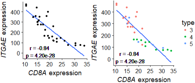
ts=cor.test(x$a,x$b); ts
str(ts)
p=ts$p.value;p #[1] 4.202888e-28
r=ts$estimate[['cor']];r#[1] -0.8427099
r0=round(r,2);r0
# 保留两位有效数字
#https://stackoverflow.com/questions/39623636/forcing-r-output-to-be-scientific-notation-with-at-most-two-decimals
p0=formatC(p, format = "e", digits = 2)
p0
#可视化结果
#plot(x$a,x$b)
library(ggplot2)
library(cowplot)
g=ggplot(data=x,aes(a,b))+
geom_smooth(method='lm', se=F)+ #se=F不要置信区间的阴影
geom_text(data=data.frame(), aes(x=16,y=15,label=paste0("r = ",r0,"\n p = ",p0)))+
theme_cowplot() + #除掉主题背景阴影
xlab( expression(paste( italic("CD8A")," expression") ) )+
ylab( expression(paste( italic("ITGAE")," expression") ) )
g+geom_point() #一般图
g+geom_point(aes(color=factor(clazz)))+ #使用分类变量后
scale_color_discrete("type")
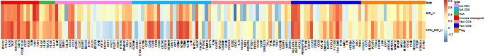
#目的: 给出数据矩阵,计算gene1和其余gene的相关系数,并画cor的heatmap。
# v0.1
#pheatmap 帮助文档 https://www.jianshu.com/p/1c55ea64ff3f

source("https://bioconductor.org/biocLite.R")
#biocLite("WGCNA")
#biocLite("ggplot2")
#biocLite("dplyr")
#biocLite("Seurat")
#biocLite("monocle")


setwd("C:\\Users\\DELL\\Desktop")


################
#read file H
msiH=read.csv("MSI-h.csv",row.names = 1)
msiH[1:3,1:3]
dim(msiH) #[1]  45 135


################
#read file
msiM=read.csv("MSIL-MSS.csv",row.names = 1)
msiM[1:3,1:3]
dim(msiM) #[1] 199 135


#check 重复项
genelist=colnames(msiM);genelist


#################
#defin function
getCorDF=function(msi){
  #cor.test
  ido1=msi$IDO1
  df=NULL
  for(i in 3:ncol(msi)){

    data2=msi[,i]
    symbol=colnames(msi)[i]

    rs=cor.test(ido1, data2)
    p=rs$p.value
    correlation=as.numeric(rs$estimate)

    tmp_df=data.frame(
      symbol=symbol,
      p=p,
      correlation=correlation
    )

    #
    df=rbind(df, tmp_df)
  }
  return(df)
}


df.h=getCorDF(msiH)
dim(df.h) #[1] 133   2
head(df.h)
row.names(df.h)=df.h$symbol
#df.h=df.h[,-1]


df.m=getCorDF(msiM)
dim(df.m) #[1] 133   2
row.names(df.m)=df.m$symbol
#df.m=df.m[,-1]
head(df.m)

cDF=data.frame(
  symbol=row.names(df.m),
  "MSI_H"=df.h$correlation,
  "NON_MSI_H"=df.m$correlation,
  row.names = 1
)
head(cDF)
dim(cDF) #[1] 133   2


########################
#heatmap
########################
library(pheatmap)

# 构建列 注释信息
type=read.csv("type.csv")
head(type)
dim(type) #[1] 133   2

annotation_col = data.frame(
  #CellType = factor(rep(c("CT1", "CT2","CT3", "CT4","CT5"), 27))
  type=type$type
)
rownames(annotation_col) = rownames(cDF)  #type$sample # paste("Test", 1:10, sep = "")
head(annotation_col)


#
# 自定注释信息的颜色列表
ann_colors = list(
  #Time = c("white", "firebrick"),
  type = c("Act CD4" = "#FF81F2", "Act CD8" = "#00B9FF","HLA" = "#39B54A",
           "immune checkpoint" = "#FF0000","Tem CD4" = "#FF8B99","Tem CD8" = "#0000FF",
           "Treg" = "#FF8000")
)
head(ann_colors)


# pheatmap
library(Cairo)
CairoPDF("sunjiaxin_10_col.pdf",width=25,height=3)
pheatmap(t(cDF), cluster_rows=F,#是否聚类 row
         cluster_cols=T, #是否聚类 列
         #display_numbers = TRUE,number_color = "blue", #标上p值

         annotation_col = annotation_col, #列 注释

         annotation_colors = ann_colors,

         angle_col=90,fontsize=10, #角度,字号
         border=FALSE #没有边框
)
dev.off()
# V2.0 修改背景颜色为白色
#http://agetouch.blog.163.com/blog/static/22853509020161194123526/
# https://www.ncbi.nlm.nih.gov/geo/query/acc.cgi?acc=GSE1323
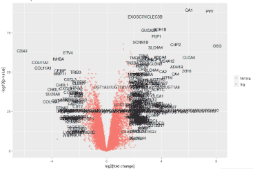
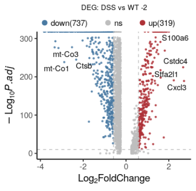
# Using ggplot2 for volcano plots 使用ggplot2画火山图
library(ggplot2)
#读取数据 #data download from GEO2R result
setwd("C:\\Users\\Administrator\\Desktop")
dif=read.table(file="Primary Tumor_Normal Colon.txt",header=T,row.names=1)
dif[1:3,1:4]
#添加显著与否标签
no_of_genes=nrow(dif);no_of_genes #4653
dif$threshold = as.factor(abs(dif$logFC) > 2 & dif$P.Value < 0.05/no_of_genes)
#画火山图
g = ggplot(data=dif, aes(x=logFC, y=-log10(P.Value), colour=threshold)) +
geom_point(alpha=0.4, size=1.75) +
#opts(legend.position = "none") +
theme(legend.title=element_blank()) +
scale_colour_hue(labels=c("Not sig.","Sig."))+
#xlim(c(-10, 10)) + ylim(c(0, 15)) +
xlab("log2[fold change]") + ylab("-log10[p-value]") +
theme_bw()+ # 背景色淡化
labs(title="Volcano plot")
g
#只标注显著基因的基因名
# 选出一部分基因:FC大且p小的基因
dd_text = dif[(abs(dif$logFC) > 2) & (dif$P.Value < 0.05/no_of_genes),]
head(dd_text)
#添加文字-基因名
g + geom_text(data=dd_text, aes(x=logFC, y=-log10(P.Value), label=dd_text$Gene.symbol), colour="black")
#为了防止遮挡,建议使用包添加文字
library(ggrepel)
g + geom_text_repel(data=dd_text, aes(x=logFC, y=-log10(P.Value), label=dd_text$Gene.symbol), colour="black")
ref: https://blog.csdn.net/wangjunliang/article/details/123093894//todo
原图 A Spatiotemporal Organ-Wide Gene Expression and Cell Atlas of the Developing Human Heart, Cell 2019 fig2D,H
脚本: volcano_singleCell_multiGroup.R
ref: https://blog.csdn.net/wangjunliang/article/details/134850344
# 加载所需的R包
library(ggplot2)
library(pheatmap)
library(reshape2)
# 读取测试数据
Input =("
Stage1_R1 Stage1_R2 Stage2_R1 Stage2_R2 Stage3_R1 Stage3_R2
Unigene0001 -1.1777172 -1.036102 0.8423829 1.3458754 0.1080678 -0.08250721
Unigene0002 1.0596877 1.490939 -0.7663244 -0.6255567 -0.5333080 -0.62543728
Unigene0003 0.9206594 1.575844 -0.7861697 -0.3860003 -0.5501094 -0.77422398
Unigene0004 -1.3553173 -1.145970 0.2097526 0.7059886 0.9516353 0.63391053
Unigene0005 1.0134516 1.445897 -0.9705129 -0.8560422 -0.2556562 -0.37713783
Unigene0006 0.8675939 1.575735 -1.0120718 -0.5856459 -0.2821991 -0.56341216
")
data = read.table(textConnection(Input), header=TRUE,row.names=1)
##
#因为数据少,所以随便倍增一些数据。真实数据请跳过这一步
data=rbind(data,data*0.8) #造数据
data=rbind(data*0.9,data*(-0.8) ) #造数据
data=rbind(data*(-0.4),data*0.6) #造数据
row.names(data)=paste0('Unigene000',seq(1:nrow(data)) )#造数据
#end
#
#data = read.table("test.txt",header = T, row.names = 1,check.names = F)
# 查看数据基本信息
head(data)#View(data)
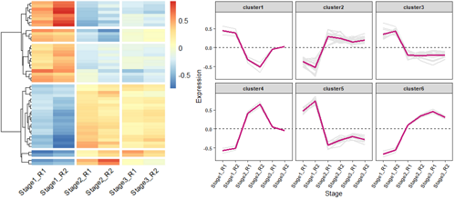
# 使用pheatmap绘制基因表达热图,并进行层次聚类分成不同的cluster
p = pheatmap(data, border=F, #不要描边
show_rownames = F, #不显示基因名
#cellwidth =40, #设置宽度
#scale ='row', #对每一行z标准化
cutree_rows = 6, #对row聚类时,设置加几个白横分割线
cluster_cols = F, #不对列聚类
gaps_col = c(2,4,6), #对列分割,仅用于不对列聚类的时候
angle_col = 45, #底部的字旋转的方向
fontsize = 12)
# 获取聚类后的基因顺序
row_cluster = cutree(p$tree_row,k=6)
# 对聚类后的数据进行重新排序
newOrder = data[p$tree_row$order,]
newOrder[,ncol(newOrder)+1]= row_cluster[match(rownames(newOrder),names(row_cluster))]
colnames(newOrder)[ncol(newOrder)]="Cluster"
# 查看重新排序后的数据
head(newOrder)
# 查看聚类后cluster的基本信息
unique(newOrder$Cluster)
#[1] 5 1 3 2 6 4
#统计每个cluster几个基因
table(newOrder$Cluster)
#1 2 3 4 5 6
#4 20 12 2 8 2
#
# 将新排序后的数据保存输出
newOrder$Cluster = paste0("cluster",newOrder$Cluster)
#write.table(newOrder, "expr_DE.pheatmap.cluster.txt",sep="\t",quote = F,row.names = T,col.names = T)
#
# 绘制每个cluster的基因聚类趋势图
newOrder$gene = rownames(newOrder)
head(newOrder)
# Stage1_R1 Stage1_R2 Stage2_R1 Stage2_R2 Stage3_R1 Stage3_R2 Cluster gene
#Unigene00032 0.4577851 0.6440856 -0.3310521 -0.2702405 -0.2303891 -0.2701889 cluster5 Unigene00032
#Unigene00033 0.3977249 0.6807646 -0.3396253 -0.1667521 -0.2376473 -0.3344648 cluster5 Unigene00033
#
#
library(reshape2)
# 将短数据格式转换为长数据格式
data_new = melt(newOrder)
head(data_new)
# Cluster gene variable value
#1 cluster5 Unigene00032 Stage1_R1 0.4577851
#2 cluster5 Unigene00033 Stage1_R1 0.3977249
# 绘制基因表达趋势折线图
ggplot(data_new,aes(variable, value, group=gene)) + geom_line(color="gray90",size=0.8) +
geom_hline(yintercept =0,linetype=2) +
stat_summary(aes(group=1),fun.y=mean, geom="line", size=1.2, color="#c51b7d") +
facet_wrap(Cluster~.) +
labs(x="Stage", y='Expression')+
theme_bw() +
theme(panel.grid.major = element_blank(), panel.grid.minor = element_blank(),
axis.text = element_text(size=8, face = "bold"),
axis.text.x=element_text(angle=60, hjust=1), #x标签旋转60度
strip.text = element_text(size = 8, face = "bold"))
#
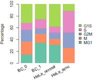
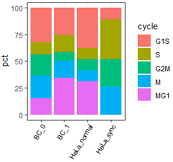
左: R原生画图; 右: ggplot2;
##data: 每群细胞中,各周期细胞数
mydatatxt="
    G1S	S	G2M	M	MG1
BC_0	28	10	17	19	13
BC_1	21	13	7	13	28
HeLa_normal	11	3	3	3	9
HeLa_sync	3	10	7	7	0
"
#从字符串中读取数据框
tbl1=read.table(text=mydatatxt, header=T) # text设置了,file就要留空
tbl1=tbl1[,c(5,4,3,2,1)] #reorder columns
tbl1
#percentage
tbl2=apply(tbl1,1,function(x){ 100*x/sum(x)})
cellNames=colnames(tbl2)
colnames(tbl2)=NULL
tbl2
#画条状图
library(RColorBrewer)
col=RColorBrewer::brewer.pal(n = 5,name = "Set2");
col=rev(col)
barplot(1:5,col=col)
#plot
par(mar=c(5, 4, 4, 5) + 0.1)
posX=barplot(as.matrix(tbl2), col=col,
        #names.arg=(paste(substr(FirstName,1,1),".",LastName)),   #设定横坐标名称
        names.arg=NULL,
        space=0.2, #条形间距
        #xlab="Individual #",
        ylab="Percentage",
        legend.text = rownames(tbl2),
        args.legend=list(x="right", #border=NA, #不要图例小方块描边
			box.col="white", inset=-0.25,bty="n"),
        border=NA)
#加底部x坐标标签
y = -0.05;
text(posX, -5, labels=cellNames, adj=1, srt=30, xpd=TRUE) #adj标签与轴的距离,srt设置xlable角度
#box()
## 使用ggplot2的版本。
mydatatxt="
    G1S	S	G2M	M	MG1
BC_0	28	10	17	19	13
BC_1	21	13	7	13	28
HeLa_normal	11	3	3	3	9
HeLa_sync	3	10	7	7	0
"
#从字符串中读取数据框
tbl1=read.table(text=mydatatxt, header=T) # text设置了,file就要留空
#转为百分数
tbl2=as.data.frame(apply(tbl1, 1, function(x){x/sum(x)*100}) )
tbl2$cycle=rownames(tbl2) #添加一列:行名
tbl2
#        BC_0      BC_1 HeLa_normal HeLa_sync cycle
#G1S 32.18391 25.609756    37.93103  11.11111   G1S

# 变为一列
dt2=reshape2::melt(tbl2,
                   id.vars='cycle', #要保留的id变量(源)
                   variable.name = "type", #melt后变量名列的名字(目标)

                   #measure.vars=c(), #要melt的变量名(列名)(源)
                   value.name="pct"); #melt后的数据列名字(目标)
head(dt2)
#  cycle type      pct
#1   G1S BC_0 32.18391
#定义图例顺序
dt2$cycle=factor(dt2$cycle, levels=c('G1S','S','G2M','M','MG1'))
ggplot(dt2, aes(x=type,y=pct, fill=cycle ))+
  geom_bar(stat='identity')+
  theme_bw()+
  #+theme(legend.position = "none")+ # 不显示坐标轴
  labs(x="")+
  theme(axis.text.x=element_text(angle=60, hjust=1,size=8,color="black") ) #坐标轴文字旋转60度
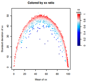
数据特点:范围是0-1,但是0.5以下很稀疏,峰值在0.8-0.9之间,1也是一个峰。
由于颜色变量偏斜太厉害,直接使用ggplot2,渐变色只能指定3种颜色,偏斜导致整体颜色太淡。
目前不会使用ggplot2设置4种颜色的渐变色,只好手动用R原生函数绘制了。
head(dif)
#	       gene	cellNumber meanDPAU	sdDPAU	      RNACounts   cpm	   totalCell	domCell	nonDomCell ratio
#RPL8	RPL8	225	99.86553	0.3462266	712259	492539.3	225	225	0	1.0000000
#RPL3	RPL3	225	99.73653	0.9470744	542531	369992.2	225	223	2	0.9911111
#...

#fig1: 查看分布图,略。
hist(dif$ratio, n=200)
abline(v=0.9, col='red', lty=2)
#

#fig2: 略。(点的颜色普遍太淡)
library(ggplot2)
ggplot(dif, aes(meanDPAU, sdDPAU, color=ratio))+
    geom_point(size=0.2)+
    scale_color_gradient2('xx\nRatio', low="navy", mid='white',  high="red", midpoint =0.7)+
    theme_bw()

#fig3: 见上图
# step0: 设置颜色。色彩向量取值范围是0-1,但是数据偏斜向1。0.5以下很稀疏。
bk0=seq(0.0,0.39,by=0.01) #almost non data
bk1=seq(0.4,0.59,by=0.01)
bk2=seq(0.6,0.79,by=0.01)
bk3=seq(0.8,1,by=0.01)
#
colors = c(
    colorRampPalette(colors = c("navy","blue"))(length(bk0)),
    colorRampPalette(colors = c("blue","#00BFFF"))(length(bk1)),
    colorRampPalette(colors = c("#00BFFF","#FFE9E9"))(length(bk2)),
    colorRampPalette(colors = c("#FFE9E9","red"))(length(bk3))
)
print( length( seq(0,1,0.01) ) )
print( length(colors) )

#
library(Cairo)
dev.off() #for jupyter bug
CairoPDF('6_9_domi__testing__.pdf', width=4.5,height=4)

#页面布局
mat = matrix(c(1,1,1,1,1,1,2,2), nrow=1, byrow=TRUE);
layout(mat)

############
#step1: plot
par(mar=c(4.5,4.5,4,0)) #bottom, left, top, right
plot(NULL, xlim=c(0,100), ylim=c(0,55), type='n',
     xlab="Mean of xx",
     ylab="Standard deviation of xx",
     main="Colored by xx ratio")
for(i in 1:nrow(dif)){
    v=round(dif$ratio[i],2)*100
    color=colors[v]
    points(dif[i,'meanDPAU'], dif[i, 'sdDPAU'],
           pch=20, cex=0.05, col=color)
}

############
#step2: 用image函数画color bar
par(mar=c(13,2.5,6,5)) #bottom, left, top, right
n=100
image(t(matrix(0:n)),col=colors,
      xaxt="n", yaxt="n", cex = 1.5,
      mgp=c(0,1,0),
      #main="Dominant\ncell ratio",
      bty='n',#box type
      xlab = "", ylab = ""
)
text(x=0,y=1.1,labels=c("xx\nratio"),xpd=T)
axis(4,at=seq(0,1,by=0.2),
     labels=seq(0,1,0.20),
     cex.axis=1, #坐标轴刻度字体大小
     #col.axis="red", #坐标轴刻度字体颜色
     #col="purple", #坐标轴颜色
     lwd=1, #坐标轴刻度粗细
     las=0)#las=0垂直于轴,2平行于轴
#
dev.off()
#cut(x, breaks): Convert Numeric to Factor

# 1. 生成数据
set.seed(20211119)
dat_1=rnorm(100, 0, 1)


# 3. 数据和颜色的映射
# fun1: 使用cut 函数,连续型变量变成分窗的因子
continuousDat2bins=function(dat, binwidth=NA){
  # to get min and max
  l1=min(dat);l1 #-1.868331
  u1=max(dat);u1 #2.796254

  l2=floor(l1*10)/10; l2 #-1.9
  u2=ceiling(u1*10)/10; u2 #2.8

  # get binwidth
  if(is.na(binwidth)){
    binwidth=(u2-l2)/100
  }

  # get breaks, include the max number
  breaks=seq(l2, u2, binwidth)
  if(max(breaks) < u2){ breaks=c(breaks, u2)}

  # convert dat to factors
  dat_3=cut(dat, breaks = breaks );
  dat_3
}
#dat_3=continuousDat2bins(dat_1)


# fun2: 分窗的因子变为渐变色颜色
bins2colors=function(bins, colors=c('green4','white','maroon3')){
  # 定义渐变色
  colors2=colorRampPalette(colors = colors, interpolate ="linear")( length(levels(bins)) )

  # map dat to colors, by index of bin index
  plotcol = colors2[ bins ];
  return(list(plotcol, colors2) )
}
#bins2colors(dat_3)

# fun3: 合并以上2个函数,连续型变量映射到渐变色颜色
continuousDat2Colos=function(dat, binwidth=NA, colors=c('green4','white','maroon3')){
  bins2colors(continuousDat2bins(dat, binwidth), colors )
}
#continuousDat2Colos(dat_1)
colors2=continuousDat2Colos(dat_1, colors=c("purple", "purple4", "black", "yellow3", "yellow"))
colors2


# 4. 画图
#pdf("01.pdf", width=3.2, height=2.8)
png("01.png", width=3.2*72, height=2.8*72, res=72)
mat=matrix(c(1,2),ncol=2)
layout(mat, widths = c(3,1)) #右图: 左右3:1

par(mar=c(3,3,1,0))
# left
plot(dat_1, pch=20,
     col=colors2[[1]],
     bty="l",
     mgp=c(2,0.8,0),
     ylab="XX value",
     main="")
box(bty="l", lwd=2) #坐标轴加粗

# right
#par(mar=c(3,1,3,5))
par(mar=c(7,0.5,2, 3))
len=length(colors2[[2]]) #颜色长度
barplot( rep(1, len), col=colors2[[2]],
         border=NA, space=0, horiz =T,
         ann=F, axes=F)

# 图例上的数字怎么能靠近整数关口? //todo
# fun: 图例表示的数值data,渐变色的长度len,获取渐变色上的刻度位置和刻度值。
getTicks=function(dat, len){ #需要手动修正
  # (Real)from min(dat) to max(dat)
  # (mark)to 0 to len
  real_tick_len=(max(dat) - min(dat)) / 4
  real_tick=seq(min(dat), max(dat), real_tick_len)
  real_tick=round(real_tick, 2)

  mark_tick=seq(0, len, (len-0)/4)
  return( list(
    label=real_tick, #等差数列,来自dat,刻度值
    at=mark_tick # 等差数列,来自渐变色长度 len,刻度位置
  ) )
}
ticks=getTicks(dat_1, len)

axis(side=4, at=ticks$at, #刻度位置
     labels=ticks$label, #刻度值
     tcl=-0.1, # 刻度线长度
     mgp=c(1,0.3,0), #刻度值与颜色条距离
     las=2)
dev.off()
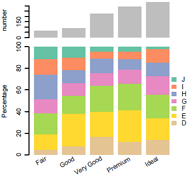
组合图,比如要求共用x坐标轴时,很难用ggplot2来处理,这时候可以考虑原生绘图,相当给力!
示例: 顶部barplot,底下百分数barplot,共用x坐标轴,所以要一一对应。
library(Cairo)
# make data
dt0=diamonds[1:1000,]
head(dt0)
dt1=table(dt0$cut, dt0$color)
dt1

CairoPDF('barplot_combine.pdf', width=4,height=4) #要在布局代码之前保存

#页面布局
mat = matrix(c(1,1,2,2,2,2), ncol=1, byrow=T);mat
layout(mat)

### fig1 barplot
dt.rsum=apply(dt1, 1, sum)
dt.rsum
par(mar=c(1,4,4,6)+ 0.1) #bottom, left, top, right
barplot(as.numeric(dt.rsum), ylab="number",
        names.arg=NULL,border=NA,space=0.2)

#### fig2 percentage barplot
tbl2=apply(dt1,1,function(x){ 100*x/sum(x)})
cellNames=colnames(tbl2)
colnames(tbl2)=NULL
tbl2
#画条状图
library(RColorBrewer)
col=RColorBrewer::brewer.pal(n = nrow(tbl2),name = "Set2");
col=rev(col)
#barplot(1:5,col=col)
#plot
par(mar=c(5, 4, 0, 6) + 0.1) ##bottom, left, top, right
posX2=barplot(as.matrix(tbl2), col=col,
             #names.arg=(paste(substr(FirstName,1,1),".",LastName)),   #设定横坐标名称
             names.arg=NULL,
             space=0.2, #条形间距
             #xlab="Individual #",
             ylab="Percentage",
             legend.text = rownames(tbl2),
             args.legend=list(x="right", border=NA, #不要图例小方块描边
                            box.col="black", inset=-0.1,bty="n"),
             border=NA)
# 加底部x坐标标签
y2 = par('usr')[3]-2;
text(posX2, y2, labels=cellNames, adj=1, srt=30, xpd=TRUE) #adj标签与轴的距离,srt设置xlable角度
#box()
dev.off()

## 绘图区域的大小
# par('usr') #c(x1, x2, y1, y2)
#[1]  -0.032   6.232  -1.000 100.000
#附: fig1 barplot 如果想在bar顶部标记上数字和百分比
dt.rsum=apply(dt1, 1, sum);dt.rsum
dt.rsum=as.numeric(dt.rsum);dt.rsum
par(mar=c(1,4,5,6)+ 0.1) #bottom, left, top, right
posX=barplot(dt.rsum, ylab="number",
        ylim=c(0,400),
        names.arg=NULL,border=NA,space=0.2)
text(x=posX, y=dt.rsum+20, label=paste0(dt.rsum, '\n(', round(dt.rsum/sum(dt.rsum),2)*100,'%)' ),
    font=1,cex=0.7)
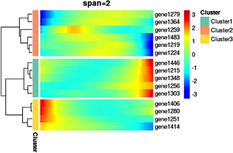
感觉调试的影响有可能大于生物学意义本身,只能看大趋势,细节的起伏很大程度上被平滑化掩盖掉了。
1.对于细胞,按照monocle等伪时间顺序排列。
2.对于基因,使用了log2(cpm+1)作为表达量,按照表达量最高的前20%细胞的中位数排序,选前几十个基因。
3.对每个基因,使用 LOESS 做平滑化后的基因表达值做heatmap。
对本模拟数据而言,span=1左右平滑化似乎最优。
目标图片 monocle at github:
分化过程图 | 2个分化方向 |
下面是本代码效果图。
 #调试和探索函数
check=function(df){
  print(dim(df))
  print(head(df))
}


# 负二项分布,模拟基因的表达,比正态分布更优。
a1=c(); a2=c()
for(i in 1:1000){
  w=rnbinom(cellNumber, size = 100, prob = 0.1)
  #plot(w)
  a1=c(a1, mean(w) )
  a2=c(a2,  sd(w))
}
plot(a1,a2)
w=rnbinom(cellNumber, size = 100, prob = 0.1)
hist(w)

############### color bar from monocle::plot_pseudotime_heatmap ##############
# 这个 color bar 来自于monocle,画热图效果很好。该渐变色原理和细节请参考 http://www.biomooc.com/R/R-color.html#2_3
# fn1
table.ramp = function (n, mid = 0.5, sill = 0.5, base = 1, height = 1) {
  x <- seq(0, 1, length.out = n)
  y <- rep(0, length(x))
  sill.min <- max(c(1, round((n - 1) * (mid - sill/2)) + 1))
  sill.max <- min(c(n, round((n - 1) * (mid + sill/2)) + 1))
  y[sill.min:sill.max] <- 1
  base.min <- round((n - 1) * (mid - base/2)) + 1
  base.max <- round((n - 1) * (mid + base/2)) + 1
  xi <- base.min:sill.min
  yi <- seq(0, 1, length.out = length(xi))
  i <- which(xi > 0 & xi <= n)
  y[xi[i]] <- yi[i]
  xi <- sill.max:base.max
  yi <- seq(1, 0, length.out = length(xi))
  i <- which(xi > 0 & xi <= n)
  y[xi[i]] <- yi[i]
  height * y
}

# fn2
rgb.tables=function (n, red = c(0.75, 0.25, 1), green = c(0.5, 0.25, 1),  blue = c(0.25, 0.25, 1)) {
  rr <- do.call("table.ramp", as.list(c(n, red)))
  gr <- do.call("table.ramp", as.list(c(n, green)))
  br <- do.call("table.ramp", as.list(c(n, blue)))
  rgb(rr, gr, br)
}

# fn3
blue2green2red=function (n) {
  rgb.tables(n, red = c(0.8, 0.2, 1), green = c(0.5, 0.4, 0.8), blue = c(0.2, 0.2, 1))
}

bks <- seq(-3.1,3.1, by = 0.1)
hmcols <- blue2green2red(length(bks) - 1)
hmcols
# view the color bar
barplot(rep(1, length(hmcols)), col=hmcols, border = NA, space=0, axes=F)


############### make data: 造数据,如果时真实数据,跳过这一步 ##############
makeData=function(){
  df=NULL
  set.seed(2020)
  for(i in 1:geneNumber){
    #a=rnorm(cellNumber, mean = 3, sd = 5)
    a=rnbinom(cellNumber, size = 1000, prob = 0.1) #负二项分布

    names(a)=paste0('cell', 1:cellNumber)
    df=rbind(df, a)
  }
  #rownames(df)=paste0('gene', 1:geneNumber)
  dim(df)
  df[1:10,1:5]

  ## 倍增仅
  df=rbind(df,df*0.8) #造数据
  df=rbind(df*1.9,df*(-1.8) ) #造数据
  df=rbind(df*(-0.4),df*0.6) #造数据
  #
  #负值变正数
  df=apply(df, 2, function(x){
    ifelse(x<0, -10*x, 10*x)
  })
  df=as.data.frame(df)
  # 要去掉全是0的行
  keep=apply(df,1,sum)>0
  df=df[keep,]
  row.names(df)=paste0('gene',seq(1:nrow(df)) )#造数据
  return(df)
}
#
cellNumber=100
geneNumber=300
df2=makeData()
dim(df2)
df2[1:10,1:5]

# normalization
df2.cpm=apply(df2, 2, function(x){1e6*x/sum(x)})
df2.log2cpm=apply(df2.cpm, 2, function(x){log2(x+1)})
dim(df2.log2cpm)
head(df2.log2cpm[,1:4])


library(pheatmap)
pheatmap( df2, scale='row')
pheatmap( df2.log2cpm, scale='row') #这热图没法看


###
## step2: select genes, by expression
#筛选前10%细胞表达median值最高的10%的基因
median_df=NULL
i=1
for(gene in rownames(df2.log2cpm)){
  i=i+1
  #if(i>10)break;

  tmp=as.numeric(df2.log2cpm[gene,])
  tmp=tmp[order(-tmp)]
  tmp.median=median(tmp[1: round(length(tmp)*0.1)])
  median_df=rbind(median_df, data.frame(
    gene=gene,
    value=tmp.median,
    sd=sd(tmp)
  ))
}
rownames(median_df)=median_df$gene
median_df=median_df[order(-median_df$value),]
check(median_df)

useGenes=rownames(median_df)[1:round(geneNumber*0.05)]
length(useGenes)
head(useGenes)

# 使用标准化后的数据
p=pheatmap(df2.log2cpm[useGenes,] , border_color = NA, scale='row',
           color=hmcols, main="log2cpm")
#使用原始counts数据
#p=pheatmap(df2[useGenes,] , border_color = NA, scale='row',
#           color=hmcols, main="raw counts")

#get cell order from heatmap, and reorder df
cellOrder=colnames(df2.log2cpm)[p$tree_col$order]
head(cellOrder)
df3=df2.log2cpm[,cellOrder]
head(df3[,1:4])

########################
## LOESS 平滑化
########################

##########
# test one gene
geneID=1
y1=df3[geneID,]
plot(y1, type='l')
#
addLine=function(span, color, ...){
  y2=predict(loess(df3[geneID,] ~ seq(1, ncol(df3)), span=span))
  lines(y2, type="l", col=color, ...)
}
addLine(0.1, 'green')
addLine(0.2, 'blue')
addLine(0.5, 'red') #差不多了
addLine(1, 'purple',lwd=2)
addLine(2, 'orange',lwd=2, lty=2)
addLine(8, 'grey',lwd=5, lty=2)

##########
## 批量化
testSpan=function(span=0.2){
  df4=apply(df3, 1, function(x){
    predict(loess(x ~ seq(1, length(x)), span=span))
  })
  df4=as.data.frame(t(df4))
  colnames(df4)=colnames(df3)
  dim(df3)
  dim(df4)
  head(df4[,1:5])

  ## heatmap again
  p=pheatmap(df4[useGenes,] , border_color = NA, scale='row',
           clustering_method='ward.D2',
           cluster_cols = F,
           show_colnames = F,
           #gaps_col = c(60),
           cutree_rows = 3,
           color=hmcols, main=paste0("span=", span) )
  return(p)
}

# test various span for perfect effect
testSpan(0.1)
testSpan(0.5)
testSpan(1) #效果可以
testSpan(1.5) #
testSpan(2) #效果可以
testSpan(4)
testSpan(8) #之后无变化
testSpan(16)
testSpan(32)
testSpan(100)
#
testSpan(0.2)
testSpan(0.3)
testSpan(0.4)
testSpan(0.5)#
testSpan(0.6)
testSpan(0.7)
testSpan(0.8)
testSpan(0.9)


# 重绘热图,add row annotation
p2=testSpan(2)
# 获取聚类后的基因顺序
row_cluster = cutree(p2$tree_row,k=3)
row_cluster
# 获取每个cluster的基因名字
gSet1=names(row_cluster[which(row_cluster==1)]) #示例
#


annote_row=data.frame(
  gene=names(row_cluster),
  Cluster=paste0("Cluster",unname(row_cluster)),
  row.names = 1
)
annote_row$Cluster=as.factor(annote_row$Cluster)
head(annote_row)

## 这个自定义颜色必须是list,不能是df!!
annote_color=list(
  Cluster=c('Cluster1'="#66C3A6", 'Cluster2'="#FD8D63",'Cluster3'="#FFD92F")
)
head(annote_row)

testSpan2=function(annote_row,annote_color, span=0.2){
  df4=apply(df3, 1, function(x){
    predict(loess(x ~ seq(1, length(x)), span=span))
  })
  df4=as.data.frame(t(df4))
  colnames(df4)=colnames(df3)
  dim(df3)
  dim(df4)
  head(df4[,1:5])

  ## heatmap again
  p=pheatmap(df4[useGenes,] , border_color = NA, scale='row',
             clustering_method='ward.D2',
             cluster_cols = F,
             show_colnames = F,
             annotation_row = annote_row,
             annotation_colors = annote_color,
             #gaps_col = c(60),
             cutree_rows = 3,
             color=hmcols, main=paste0("span=", span) )
  return(p)
}
testSpan2(annote_row,annote_color, span=2) #页码上面的示例图就是这一步的结果
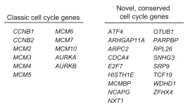
目标图片: 2015 Cell, Drop seq, Figure 4 Cell-Cycle Analysis of HEK and 3T3 Cells Analyzed by Drop-Seq.
细胞周期相关基因 list: A complete list of cell-cycle regulated genes can be found in
Table S2.zip Or
txt
原文是一段非常高质量的R代码,充分展示了如何嵌套使用apply家族函数、如何函数嵌套、如何定义输入和输出。
下文为了方便理解,把原来的嵌套函数拆开了。
# aim: scRNAseq to determine cell cycle.
# 缺陷: 这是对细胞系做的周期分类,没有考虑G0期。
# source: 2015 cell, drop seq;
# v0.3 fix filter line.
## 准备工作
#1. 定义资源的路径: infoPath
infoPath="/home/wangjl/data/cellLines/"
#basic information, like cycle gene list, RNA expression matrix, cell type info;
#2.下载周期相关基因列表,命名为 G1S.txt等5个文件,一个基因一行,不加引号。文件放到infoPath下。
#3. 你自己的单细胞转录组表达矩阵, row为基因,column为cell;
#4. cell information: 可选参数,用于对表达矩阵的column做筛选,也就是取细胞的子集。
# 经验:
#1. 一次对一种细胞做细胞周期鉴定,超过一个种类可能结果不准确;
#2. 如果细胞的一部分是(药物、刺激等)处理过的,那么用normal部分筛选基因后,对全部细胞做周期鉴定,否则会失真。
#3. 要保证矩阵不能有全是0的行。本例是3'测序,使用的是log(cpm+1),如果是全长测序,可以使用log(tpm+1)或log(rpkm+1)
setwd("/home/wangjl/data/cellLines/cycle/")
outputRoot="BC_"
#load data: 表达counts矩阵 (确定是 raw counts矩阵,第一步过后会有标准化)
fname=paste0(infoPath,"BC_HeLa.225cells.count.V3.csv")
data=read.csv(fname,row.names = 1)
dim(data) #[1] 18679 225
data[1:4,1:4]
# c01ROW24 c01ROW35 c01ROW31 c05ROW02
#A1BG-AS1 0 0 0 0
#A2M 0 0 0 0
#helper: return cell phase names
getCellPhaseList=function(){
c('G1S', 'S','G2M','M','MG1');
}
#load data: 细胞类型
cellType=read.csv( paste0(infoPath,"cellInfo.txt"),row.names = 1)
head(cellType)
# geneNumber countsPerCell countsPerGene cellType
#c01ROW24 5693 1950601 342.6315 BC_syncMix
#c01ROW35 6768 3048970 450.4979 BC_syncMix
dim(cellType) #225 4
#获取细胞子集:BC
data2=data[,row.names(cellType[which( substr(cellType$cellType,1,3)=="BC_" ),])]
dim(data2) #[1] 18679 169
#只保留非0的行
keep=apply(data2>0,1,sum)>0
table(keep)
#FALSE TRUE
#403 18276
data2=data2[keep,] #filter out all 0 rows
dim(data2) #[1] 18276 169
#load data: 每个时期的gene set,和表达矩阵求基因交集
geneSets=list();
for(i in 1:length(getCellPhaseList() )){
setName=getCellPhaseList()[i]
print( paste(i, setName) )
tmpGenes=readLines( paste0(infoPath,setName,'.txt') )
print( length(tmpGenes) )
#和矩阵的列求交集
geneSets[[setName]]=intersect(tmpGenes, row.names(data2))
print( length(geneSets[[setName]])) #95
}
## begin
#step1: exclude genes cor<0.3 with mean of the set
geneSets2=list();
for(i in 1:length(getCellPhaseList() )){
#求G1S集合中的gene mean
setName=getCellPhaseList()[i] #'G1S';
print( paste(i, setName) )
setMean=apply(data2[geneSets[[setName]], ], 2,mean)
#head(setMean)
#每个基因和平均值求cor
tmpGenes=c()
for(g in geneSets[[setName]]){
#rs=cor(t(data2[g,]), setMean)
rs=cor(as.numeric(data2[g,]), setMean)
#print( paste(g,rs) )
if(rs>=0.3){
tmpGenes=c(tmpGenes,g)
}
}
#[1] "ACD 0.324866931495592"
#[1] "ACYP1 0.0858240480040331"
#[1] "ADAMTS1 -0.128818193750771"
print( length(tmpGenes) )
geneSets2[[setName]]=tmpGenes
}
geneSets2
sum(sapply(geneSets2, function(x){length(x)})) #321
# step2: depth norm; log2 norm;
getNormalizedCts <- function ( cts ) {
#ctsPath
#cts <- read.table ( ctsPath , header = T , as.is = T )
apply ( cts , 2 , function ( x ) { log2 ( ( 10^6 ) * x / sum ( x ) + 1 ) })
}
normCts=getNormalizedCts(data2)
dim(normCts)
normCts[1:10,1:5]
#apply(normCts,2,sum)
#step3: calculate 5 phase scores each cell(mean of phase genes)
# Tested. Passed.
assignSampleScore <- function ( phaseGenesList , normCts ) {
scores <- lapply ( phaseGenesList , function ( pGenes ) {
print(length(pGenes) )
apply ( normCts , 2 , function ( x ) {
mean ( x [ pGenes ] )
} )
} )
do.call ( cbind , scores )
}
scoreMatrix <- assignSampleScore ( geneSets2 , normCts )
dim(scoreMatrix) #169 5
head(scoreMatrix)
# G1S S G2M M MG1
#c12ROW02 3.774424 3.742809 3.131765 3.524596 4.595119
#c12ROW03 3.274414 2.999720 3.231767 3.422519 5.221042
write.table ( scoreMatrix , paste ( outputRoot , "PhaseScores.txt" , sep = "" ) )
# pheatmap(scoreMatrix, scale='row', border_color = NA)
#step4: z-norm(each phase, then each cell)
# Tested. Passed.
getNormalizedScores <- function ( scoreMatrix ) {
norm1 <- apply ( scoreMatrix , 2 , scale )
normScores <- t ( apply ( t ( norm1 ) , 2 , scale ) )
rownames ( normScores ) <- rownames ( scoreMatrix )
colnames ( normScores ) <- colnames ( scoreMatrix )
normScores
}
normScores <- getNormalizedScores ( scoreMatrix )
head(normScores)
# G1S S G2M M MG1
#c12ROW02 -0.5587886 1.71406144 -0.767616785 0.012780937 -0.4004370
#c12ROW03 -1.0458011 -0.56059069 -0.005651298 0.002073499 1.6099696
write.table ( normScores , paste ( outputRoot , "PhaseNormScores.txt", sep = "" ) )
#pheatmap(normScores, scale='row', border_color = NA)
#画出每个细胞的各个周期打分
i=5;plot(normScores[i,],type='o',col=rainbow(i), main=rownames(normScores)[i])
i=8;plot(normScores[i,],type='o',col=rainbow(i), main=rownames(normScores)[i])
#step5: assign phase for each cell
getReferenceProfiles <- function () {
referenceProfiles <- list (
"G1S" = c ( 1 , 0 , 0 , 0 , 0 ) ,
"G1S.S" = c ( 1 , 1 , 0 , 0 , 0 ) ,
"S" = c ( 0 , 1 , 0 , 0 , 0 ) ,
"S.G2M" = c ( 0 , 1 , 1 , 0 , 0 ) ,
"G2M" = c ( 0 , 0 , 1 , 0 , 0 ) ,
"G2M.M" = c ( 0 , 0 , 1 , 1 , 0 ) ,
"M" = c ( 0 , 0 , 0 , 1 , 0 ) ,
"M.MG1" = c ( 0 , 0 , 0 , 1 , 1 ) ,
"MG1" = c ( 0 , 0 , 0 , 0 , 1 ) ,
"MG1.G1S" = c ( 1 , 0 , 0 , 0 , 1 ) ,
"all" = c ( 1 , 1 , 1 , 1 , 1 ) )
#referenceProfiles <- lapply ( referenceProfiles , function ( x ) { names ( x ) <- c ( "G1S", "S", "G2" , "G2M" , "MG1" ); x } )
referenceProfiles <- lapply ( referenceProfiles , function ( x ) {
names ( x ) <- c ( 'G1S', 'S','G2M','M','MG1' ); x } )
do.call ( rbind , referenceProfiles )
}
# Tested. Passed.
assignRefCors <- function ( normScores ) {
referenceProfiles <- getReferenceProfiles()
t ( apply ( normScores , 1 , function ( sampleScores ) {
apply ( referenceProfiles , 1 , function ( refProfile ) {
cor ( sampleScores , refProfile ) } )
} ) )
}
# Tested. Passed.
getPhases <- function ( ) {
#phases <- c ( "G1S", "S", "G2" , "G2M" , "MG1" )
phases <- c ( 'G1S', 'S','G2M','M','MG1' )
names ( phases ) <- phases
phases
}
# Tested. Passed.
assignPhase <- function ( refCors ) {
phases <- getPhases ()
apply ( refCors [ ,phases ] , 1 , function ( x ) {
phases [ which.max ( x ) ]
} )
}
###### Score cycle similarity
refCors <- assignRefCors ( normScores )
head(refCors)
assignedPhase <- assignPhase ( refCors )
head(assignedPhase)
#
table(assignedPhase)
# assignedPhase
#G1S G2M M MG1 S
#49 24 32 41 23
#
getDFfromNamed=function(Namedxx){
data.frame(
id=attr(Namedxx,'names'),
val=unname(Namedxx),
row.names = 1
)
}
rs=getDFfromNamed(assignedPhase)
head(rs)
#保存标签结果
write.csv(rs,paste ( outputRoot , "cellCycle_phase.csv" , sep = "" ) )
#
#和第四步比较呢?
i=5;plot(normScores[i,],type='o',col=rainbow(i), main=rownames(normScores)[i])
#目测几个,就是求最高值
#
#step6 ####### Order cells
# Tested. Passed.
orderSamples <- function ( refCors , assignedPhase) {
phases <- getPhases()
orderedSamples <- list()
for ( phase in phases ) {
phaseCor <- refCors [ assignedPhase == phase , ]
phaseIndex <- which ( colnames ( phaseCor ) == phase )
if ( phaseIndex == 1 ) { preceding = ncol ( phaseCor ) - 1 } else { preceding <- phaseIndex - 1 }
if ( phaseIndex == ncol ( phaseCor ) - 1 ) { following = 1 } else { following <- phaseIndex + 1 }
earlyIndex <- phaseCor [ , preceding ] > phaseCor [ , following ]
earlyCor <- subset ( phaseCor , earlyIndex )
earlySamples <- rownames ( earlyCor ) [ order ( earlyCor [ , preceding ] , decreasing = T ) ]
lateCor <- subset ( phaseCor , ! earlyIndex )
lateSamples <- rownames ( lateCor ) [ order ( lateCor [ , following ] , decreasing = F ) ]
orderedSamples [[ phase ]] <- c ( earlySamples , lateSamples )
}
refCors [ do.call ( c , orderedSamples ) , ]
}
#
ordCor <- orderSamples ( refCors , assignedPhase )
write.table ( cbind ( ordCor , "assignedPhase" = assignedPhase [ rownames ( ordCor ) ] ) ,
paste ( outputRoot , "PhaseRefCor.txt" , sep = "" ) )
#
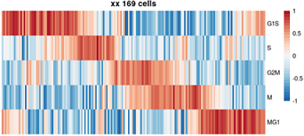
#step7 ####### Plot
# Passed.
plotCycle <- function ( phaseCorsMatrix, ... ) {
library("pheatmap")
library("RColorBrewer")
breaks <- seq ( -1 , 1 , length.out = 31 )
heatColors <- rev (brewer.pal ( 9, 'RdBu'))
heatColors <-colorRampPalette(heatColors)
colorPallete <- heatColors((length ( breaks ) - 1 ))
# create heatmap
hm.parameters <- list(phaseCorsMatrix, border_color=NA,
color = colorPallete,
breaks = breaks,
cellwidth = NA, cellheight = NA, scale = "none",
treeheight_row = 50,
kmeans_k = NA,
show_rownames = T, show_colnames = F,
#main = "",
clustering_method = "average",
cluster_rows = FALSE, cluster_cols = FALSE,
clustering_distance_rows = "euclidean",
clustering_distance_cols = NA ,
legend = T , annotation_legend = F,... )
do.call("pheatmap", hm.parameters )
}
phases <- getPhases()
#jpeg ( paste ( outputRoot , "PhasePlot.jpg" , sep = "" ) , 5 , 3 , units = "in" , res = 300 )
pdf( paste0( outputRoot, "a7_PhasePlot.pdf"), width=4, height=2.5)
plotCycle ( t ( ordCor [ , phases ] ), main= paste0("XX ", nrow(ordCor), ' cells') )
#dev.off()
## check
df1=rs
head(df1)
table(df1$val)
cellType2=cellType[rownames(df1),]
cellType2$cellCycle=df1$val
head(cellType2)
table(cellType2$cellType, cellType2$cellCycle)
# G1S G2M M MG1 S
#BC_0 28 17 19 13 10
#BC_1 21 7 13 28 13
目标图片: Science 2018, Fig. 5 The molecular clock across tissues
(C) Distribution of the peak phases of core clock components in the tissues where they are detected as cycling.
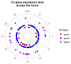
#1. make data
n=200
set.seed(10)
dt=data.frame(
  time=runif(n, 0,24),
  gene1=rbinom(n, 1, 0.1),
  gene2=rbinom(n, 1, 0.4),
  gene3=rbinom(n, 1, 0.1)
)

dt[which(dt$gene1==1),]$gene1=7
dt[which(dt$gene2==1),]$gene2=7.5
dt[which(dt$gene3==1),]$gene3=9
#table(dt$gene3)
library(reshape2)
df=melt(dt, id="time")
head(df)
# 第一列时间点(0-24), 第二列基因名字,第三列基因表达是与否(0或1)
#    time     variable  value
#1 12.179477    gene1     0
#2  7.362444    gene1     0
#3 10.245784    gene1     0

#2. draw
draw=function(df){
  #step1 定义一个无数据的空坐标系统
  g=ggplot()+
    theme_bw()+
    theme(panel.grid =element_blank(), ## 删去网格线
          panel.border = element_blank(), #去掉外边框
          plot.title = element_text(hjust = 0.5), #标题居中
          axis.text.y = element_blank(), #删掉y轴文字
          axis.ticks = element_blank() #删去坐标刻度
          ) +
    #coord_cartesian(ylim=c(1.5,2.8))+
    scale_y_continuous( expand = c(0,0), #去掉图与y轴间隙
                       limits=c(5,10))+ #y轴显示范围
    scale_x_continuous(expand = c(0,0),
                       breaks=seq(0,24,2), #每2个一个刻度
                       labels=seq(0,24,2))+
    labs(x="", y="", title="XX gene expression level\nacross the hours")

  #step2 添加网格线: 放射线
  g=g + geom_vline(aes(xintercept= seq(0,24,2) ), color="#D0D0D0", size=0.8,
                   linetype="dashed")

  #step3 添加网格线: 圆圈线
  for(i in c( 7, 7.5, 9)){
   g=(function(i2){
     print(i2)# 不加这一句不更新,会遇到闭包问题
     g + geom_hline(aes(yintercept=i2), color="#DFDFDF", size=1,
                    linetype="dashed")
   })(i)
  }
  g=g + geom_hline(aes(yintercept=c(6,10) ), color="#DFDFDF", size=1,
                linetype="solid")
  #step4 添加数据
  g=g+geom_point(mapping= aes(time, value, fill=variable),
                 shape=21, color="NA", size=3,
                 data=df)+
    scale_fill_manual('XX Gene', values = c('red', 'blue', 'purple'))+
    geom_rect(data = NULL, # 中心圆环
              aes(ymin = 5,  ymax = 5.9),
              xmin = -Inf, xmax = Inf,
              fill = "white", colour = "white", size = 1,
              linetype="solid")
  return(g)
};draw(df)+coord_polar()
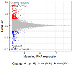
head(df3) #数据 7776    5
#        mean_normal mean_sync     mean     delta status
#SPARC    0.02001691  3.917605 1.866243 -4.884748   down
#COX5BP1  0.01877168  4.004604 1.906797 -4.871463   down

#求平均数和标准差
m1=mean(df3$delta)
sd1=sd(df3$delta)
# 统计status列每个值的个数
tb=table(df3$status);tb
#down   ns   up
# 124 7454  198

#ggplot2 画图
g=ggplot(df3, aes( x= mean , y=delta, color=factor(status,levels=c('up','ns','down')) ) ) +
  geom_point(alpha=0.5,size=0.1)+
  labs( title="xxx", x='Mean log RNA expression', y="Delta CV" ) + theme_bw()+
  theme(legend.box = "horizontal", # 图例,水平,标到底部
        legend.key.size=unit(10,"pt"), #图例方块的高度
        legend.position="bottom") +
  scale_color_manual('Change', labels=c( paste0("up(",tb[3],")"),paste0('n.s.(',tb[2],')'),paste0("down(",tb[1],")") ), #图例文字
                     values=c("red", "grey",'blue') )+ #自定义颜色
  #scale_shape(guide = guide_legend(title.position = "top", size=12)) +
  geom_hline(aes(yintercept=m1+sd1*2), color="#aaaaaa", linetype="dashed")+
  geom_hline(aes(yintercept=m1-sd1*2), color="#aaaaaa", linetype="dashed");g

# 为点添加文字注释
library(ggrepel)
dd_text=df3[which(df3$delta >m1+sd1*7 | df3$delta < (m1-sd1*8) ),];dim(dd_text)
g2=g+geom_text_repel(data=dd_text, aes(x=mean, y=delta, label=rownames(dd_text)),
                  color="black",size=3,alpha=0.6)+
  guides(colour = guide_legend(override.aes = list(alpha = 1,size=2)))#放大图例的点
# 保存到文件
library(Cairo)
CairoPDF(file="03_RNA_Sync_vs_normal_HeLa_CV_changed_genes_v3.pdf",width=4,height=4)
print(g2)
dev.off()
可以使用 text()
或使用 ggplot2 的 geom_text() 和 geom_label(), 参考实现 4_3。
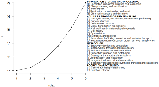
# 读取文件
text1=read.delim("fun.txt",header=FALSE) #该文件在文末
text1
len=nrow(text1); #29
b=20;

# 绘图
#tiff(filename="haha.tif",width=25,height=12,units="cm",compression="lzw",bg="white") #?
#png(file="aaaa.png",width=800,height=600);
#svg('aaaa.svg', width=8, height=6)

pdf('aaaa.pdf', width=10, height=6)
# 左边的图
par(fig=c(0,0.55,0,1),bty="n");
plot(c(0,1,4,9,16,25), type='o',ylab="y", pch=20)

# 右边的图: 文字
par(fig=c(0.4,1,0,1),bty="n", new=TRUE); #fig=c(x1, x2, y1, y2), 添加到新图 new = TRUE
plot(1:b,1:b,type="n", #type="n"不生成任何点和线,创建坐标系
     xaxt="n",yaxt="n",
     xlab="",ylab="");
sum=b+b/(2*len); #20.3448
for(i in 1:(len)){
  if (i %in% c(1,7,18,27) ){
    text(1,sum,text1[i,],adj=0,cex=0.8,font=2); #大号字体
  }else{
    text(1,sum,text1[i,],adj=0,cex=0.8, col='grey20')
  }
  sum=sum-b/(len); #一行的高度差不多是 20/1.6896
  print(sum)
}
dev.off()


####### 补充材料
$ cat fun.txt
INFORMATION STORAGE AND PROCESSING
[J] Translation, ribosomal structure and biogenesis
[A] RNA processing and modification
[K] Transcription
[L] Replication, recombination and repair
[B] Chromatin structure and dynamics
CELLULAR PROCESSES AND SIGNALING
[D] Cell cycle control, cell division, chromosome partitioning
[Y] Nuclear structure
[V] Defense mechanisms
[T] Signal transduction mechanisms
[M] Cell wall/membrane/envelope biogenesis
[N] Cell motility
[Z] Cytoskeleton
[W] Extracellular structures
[U] Intracellular trafficking, secretion, and vesicular transport
[O] Posttranslational modification, protein turnover, chaperones
METABOLISM
[C] Energy production and conversion
[G] Carbohydrate transport and metabolism
[E] Amino acid transport and metabolism
[F] Nucleotide transport and metabolism
[H] Coenzyme transport and metabolism
[I] Lipid transport and metabolism
[P] Inorganic ion transport and metabolism
[Q] Secondary metabolites biosynthesis, transport and catabolism
POORLY CHARACTERIZED
[R] General function prediction only
[S] Function unknown
怎么让GO分析结果更高大上呢?
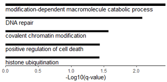
 #数据源是 metascape 做的GO分析结果: http://www.metascape.org/

# install.packages('xlsx')
loadGOfromXLS=function(fname){
  library(xlsx)
  dat = read.xlsx(fname, sheetName = "Enrichment", encoding = 'UTF-8')
  #dim(dat) #164 9
  # (1)filter by p value
  dt2=dat[which(dat$Log.q.value. < log10(0.05)),]
  head(dt2[,c(1,2,3,6)])
  #dim(dt2) #17 9
  #colnames(dt2)
  #1."GroupID"       "Category"      "Term"     "Description"   "LogP"          "Log.q.value."
  #7 "InTerm_InList" "Genes"         "Symbols"

  # (2)filter out duplicate terms
  dt3=dt2[!duplicated(dt2[,'Description']),]
  # (3) keep Summary only
  dt4=dt3[grep('Summary',dt3$GroupID),]
  return(dt4)
}

library(ggplot2)
GO_barplot=function(dt0){
  dt0=dt0[order(-dt0$Log.q.value.),]
  ggplot(dt0, aes(x=Description, y=-Log.q.value.
                  #, fill=Category
                  ))+
    geom_bar(stat="identity", width=0.15, fill="black")+
    coord_flip()+
    scale_x_discrete(limits=dt0$Description,labels = NULL )+
    theme_classic()+
    theme(legend.position="none")+
    scale_y_continuous(expand = c(0,0))+ #去掉坐标轴两端的空白
    annotate("text", x=seq(1, nrow(dt0))-0.3, y=0, #位置
             hjust = 0, #文字左对齐
             label= dt0$Description)+
    labs(x="", y="-Log10(q-value)")+
    theme( axis.ticks.y = element_blank(),
           axis.line.y = element_blank(),
           axis.text.y = element_blank() )
}

# read and plot
fname="F:\\c1_Figure\\Fig2\\vstVar_changed_HeLa\\down-313\\all.tfo2sgtfh\\metascape_result.xlsx"
dt4=loadGOfromXLS(fname)
GO_barplot(dt4)


# or plot using part of these items.
g2=GO_barplot(dt2[c(seq(1,8), 11,15,16,18,19,20),])
g2

## save to pdf
library(Cairo)
CairoPDF(file='F:/c1_Figure/GO_replot/06_CCNB1-pearson_cor-89genes.pdf',width=7,height=5)
g2
dev.off()
水平barplot,带前n个基因列表。效果图见 csdn 。
loadGOfromXLS=function(fname){
  library(xlsx)
  dat = read.xlsx(fname, sheetName = "Enrichment", encoding = 'UTF-8')
  #dim(dat) #164 9
  # (1)filter by p value
  dt2=dat[which(dat$Log.q.value. < log10(0.05)),]
  head(dt2[,c(1,2,3,6)])
  #dim(dt2) #17 9
  #colnames(dt2)
  #1."GroupID"       "Category"      "Term"     "Description"   "LogP"          "Log.q.value."
  #7 "InTerm_InList" "Genes"         "Symbols"

  # (2)filter out duplicate terms
  dt3=dt2[!duplicated(dt2[,'Description']),]
  # (3) keep Summary only
  dt4=dt3[grep('Summary',dt3$GroupID),]
  return(dt4)
}

#' re-plot GO plot as barplot with gene list
#'
#' @param dt0 data.frame from metascape excel: loadGOfromXLS()
#' @param spaceToX space to X axis
#' @param spaceToY space to Y axis
#' @param n_gene show gene number
#' @param colors color list for filling bars and text
#' @param without_category filter out those in Category
#' @param select_rows which rows to draw barplot
#' @param main the title for this figure
#'
#' @return ggplot2 object
#' @export
#'
#' @examples
GO_barplot_withGenes=function(dt0, #excel读入的数据
                              spaceToX=0.2/5, #文字和x轴的缝隙
                              spaceToY=0.1/0.2, #文字和y轴的缝隙
                              n_gene=6, #最多显示的基因个数
                              colors=NULL, #填充颜色
                              without_category=c("WikiPathways"), #去掉某些类
                              select_rows=NULL, #选择哪几行GO画图
                              debug=F,
                              main="Enrichment of PC1"
  ){
  # 1.select columns
  dat4=dt0[, c("Log.q.value.", "Description", "Category", "Term", "Symbols")]
  dat.use=dat4 #[, c("LogQvalue", "Description", "GroupID", "Symbols")]
  dat.use$LogQvalue=dat4$Log.q.value.
  dat.use$GroupID=dat4$Category

  # 2.仅显示不超过n=5个基因
  #n_gene=6 #最多保留的基因个数
  dat.use$Symbols2=sapply(dat.use$Symbols, function(x){
    arr=strsplit(x, ",")[[1]]
    len=ifelse(length(arr)>n_gene, n_gene, length(arr));
    arr=arr[1:len]
    paste0(arr, collapse = ",")
  }) |> as.character()

  # 3.filter by Category
  dat.use=dat.use[which(!dat.use$GroupID %in% without_category),]
  print(table(dat.use$Category))

  # 4.set y order: as factor
  dat.use$Description=factor(dat.use$Description)

  # 5.set colors
  #cols=c("#D51F26","#00A08A","#F2AD00","#F98400","#5BBCD6")
  n_cat=length(unique(dat.use$Category))
  if(!is.null(colors)){
    if(length(colors) < n_cat)
      warning("Provide color number < needed categories! use default color set!")
    else{
      cols=colors
    }
  }else if( n_cat<=5 ){
    cols=c("KEGG Pathway"="#D51F26",
           "GO Biological Processes"="#00A08A",
           "Reactome Gene Sets"="#F2AD00",
           "Canonical Pathways"="#F98400",
           "WikiPathways"="#5BBCD6")
  }else{
    cols=scales::hue_pal()(n_cat)
  }

  # 6.combine Term and Desc
  dat.use$Description=sprintf("(%s)%s", dat.use$Term, dat.use$Description)
  if(debug==T){
    dat.use$Description=paste(1:nrow(dat.use), dat.use$Description)
  }

  # 7.选择所需要的行 select rows to draw
  dat.use2=dat.use;
  # select rows
  if(!is.null(select_rows)){
    dat.use=dat.use[select_rows,]
  }

  ############ Plot
  library(ggplot2)
  ggplot(dat.use, aes(x=-LogQvalue, y = Description, fill = GroupID)) +
    #1. barplot of GO Q value
    geom_bar(stat ="identity", width =0.5) +
    geom_text(aes(x=spaceToY, #文字和y轴的缝隙
                  y=Description, label=Description),
              size=4,
              #fontface="bold",
              hjust=0) +
    scale_fill_manual(values = cols)+ #bar plot fill color
    scale_x_continuous(expand = c(0,0))+ #bar和y轴无间隔
    #2. add gene list
    geom_text(data = dat.use,
              aes(x =spaceToY, #文字和y轴的缝隙
                  y = Description,
                  label = Symbols2, #基因列表
                  color = GroupID),
              size =3.5,
              fontface ='italic',
              hjust =0,
              vjust =2.3) +
    scale_color_manual(values=cols) + #gene list text colors
    #3. theme and style
    theme_classic(base_size = 14)+
    theme(axis.text.y = element_blank(), #no y title, ticks, text
          axis.title.y = element_blank(),
          axis.ticks.y = element_blank(),
          axis.line = element_line(colour ='black', linewidth =1),
          axis.text.x = element_text(colour ='black', size =12),
          axis.ticks.x = element_line(colour ='black', linewidth = 1),
          axis.title.x = element_text(colour ='black', size =12),
          plot.title = element_text(size = 12),
          legend.position ="none")+ #no legend
    scale_y_discrete( #expand = c(0.2, 0), #为bar下的字符留空间,缺点是上面也有空间了
      expand=expansion(mult = c(spaceToX, 0)), #ggplot 3.5.1
      limits=rev( dat.use$Description)  #设置bar的顺序
    ) +
    labs(x="-Log10(Qvalue)", title=main)
}

# 实例
fname="E:\\research\\scPolyA-seq2\\GO-sig-with-PC\\sig-with-PC3\\all.trp87ruab\\metascape_result.xlsx"
dt4=loadGOfromXLS(fname) #函数见上文 14
GO_barplot(dt4)

p1=GO_barplot_withGenes(dt4,
                        select_rows=c(1,2,3,4,5,6,8,9,15,16),
                        debug=F,
                        spaceToX=0.2/2.5,
                        spaceToY=0.1/0.5,
                        main="Genes associated with PC3(p.adj<0.01, n=485)"); p1

pdf( paste0(outputRoot, "withPC3.pdf"), width=4.5, height=4.8)
print(p1)
dev.off()
水平浅色barplot,不带基因列表。效果图见: 14_2 csdn链接。
GO_barplot_withNoGenes=function(dt0, #excel读入的数据
                                spaceToX=0.2/5, #文字和x轴的缝隙
                                spaceToY=0.1/0.2, #文字和y轴的缝隙
                                n_gene=6, #最多显示的基因个数
                                colors=NULL, #填充颜色
                                without_category=c("WikiPathways"), #去掉某些类
                                select_rows=NULL, #选择哪几行GO画图
                                debug=F, #调试模式:打印GO 编号和序号
                                bg.alpha=0.3, #背景色的不透明度
                                main="Enrichment of PC1"
){
  # 1.select columns
  dat4=dt0[, c("Log.q.value.", "Description", "Category", "Term")]
  dat.use=dat4 #[, c("LogQvalue", "Description", "GroupID")]
  dat.use$LogQvalue=dat4$Log.q.value.
  dat.use$GroupID=dat4$Category
  # 2.保留前5个基因:略过

  # 3.filter by Category
  dat.use=dat.use[which(!dat.use$GroupID %in% without_category),]
  print(table(dat.use$Category))

  # 4.set y order: as factor
  dat.use$Description=factor(dat.use$Description)

  # 5.set colors
  #cols=c("#D51F26","#00A08A","#F2AD00","#F98400","#5BBCD6")
  n_cat=length(unique(dat.use$Category))
  if(!is.null(colors)){
    if(length(colors) < n_cat)
      warning("Provide color number < needed categories! use default color set!")
    else{
      cols=colors
    }
  }else if( n_cat<=5 ){
    cols=c("KEGG Pathway"="#D51F26",
           "GO Biological Processes"="#00A08A",
           "Reactome Gene Sets"="#F2AD00",
           "Canonical Pathways"="#F98400",
           "WikiPathways"="#5BBCD6")
  }else{
    cols=scales::hue_pal()(n_cat)
  }

  # 6.combine Term and Desc: in debug mode
  if(debug==T){
    dat.use$Description=sprintf("(%s)%s", dat.use$Term, dat.use$Description)
    dat.use$Description=paste(1:nrow(dat.use), dat.use$Description)
  }

  # 7.选择所需要的行 select rows to draw
  dat.use2=dat.use;
  # select rows
  if(!is.null(select_rows)){
    dat.use=dat.use[select_rows,]
  }

  ############ Plot
  library(ggplot2)
  ggplot(dat.use, aes(x=-LogQvalue, y = Description, fill = GroupID)) +
    #1. barplot of GO Q value
    geom_bar(stat ="identity", width =0.7, alpha=bg.alpha) +
    geom_text(aes(x=spaceToY, #文字和y轴的缝隙
                  y=Description, label=Description),
              size=4,
              #fontface="bold",
              hjust=0) +
    scale_fill_manual(values = cols)+ #bar plot fill color
    scale_x_continuous(expand = c(0,0))+ #bar和y轴无间隔

    #3. theme and style
    theme_classic(base_size = 14)+
    theme(axis.text.y = element_blank(), #no y title, ticks, text
          axis.title.y = element_blank(),
          axis.ticks.y = element_blank(),
          axis.line = element_line(colour ='black', linewidth =1),
          axis.text.x = element_text(colour ='black', size =12),
          axis.ticks.x = element_line(colour ='black', linewidth = 1),
          axis.title.x = element_text(colour ='black', size =12),
          plot.title = element_text(size = 12),
          legend.position ="none")+ #no legend
    scale_y_discrete( #expand = c(0.2, 0), #为bar下的字符留空间,缺点是上面也有空间了
      expand=expansion(mult = c(spaceToX, 0)), #ggplot 3.5.1
      limits=rev( dat.use$Description)  #设置bar的顺序
    ) +
    labs(x="-Log10(Qvalue)", title=main)
}

fname="E:\\research\\scPolyA-seq2\\GO-sig-with-PC\\sig-with-PC1\\all.t_kfvpcyl\\metascape_result.xlsx"
dt4=loadGOfromXLS(fname)
GO_barplot(dt4)

p1=GO_barplot_withNoGenes(dt4,
                          select_rows=c(1,2,4,5,6,7,9,10,16,17),
                          debug=F,
                          spaceToX=0.2/2.5,
                          spaceToY=0.2/0.5,
                          main="Genes correlated with PC1(p.adj<0.01, n=1294)"); p1

pdf( paste0(outputRoot, "withPC1-noGene.pdf"), width=4, height=3.5)
print(p1)
dev.off()
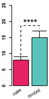
左: barplot 添加error bar;
右: line plot 添加error bar; 对坐标轴axis和轴标题、刻度标签间的距离、刻度长度的控制。
# R base 版 barplot
data = data.frame(mean = c(8, 15), sd = c(9, 17))
rownames(data) = c("case", "control")

par(lwd = 2)
xPos = barplot(data$mean, col =c('#e82364', '#5bc4ba'), #c("red", "blue"),
               ylim = c(0, 25), axes = F, font = 2)
b=xPos
text(x=xPos, y=-1.2, labels=rownames(data),
     xpd=TRUE, #允许绘制在绘图区外
     adj=1, #adj=1右上对齐
     srt=30) #倾斜30度

arrows(xPos[1], data$mean[1], b[1], data$sd[1], angle = 90) # error bar
arrows(xPos[2], data$mean[2], b[2], data$sd[2], angle = 90) # error bar

# 顶上的虚线
lines( x = c(b[1], b[1], b[2], b[2]), y = c( data$sd[1] * 1.05 , data$sd[2] * 1.1,  data$sd[2] * 1.1, data$sd[2] * 1.05), lty = 2)
# 星号
text( x = b[1] + (b[2] - b[1]) / 2, y = data$sd[2] * 1.1, label = "****", cex = 2, adj = c(0.5, 0))
# 加坐标轴
axis(side = 2, lwd = 2, font = 2, cex = 1.5)
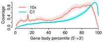
# R base 版: line plot
# 输入数据是均值和标准差
> head(dfB2)
         mean          sd
1 0.000000000 0.000000000
2 0.008797837 0.001955405
3 0.020597459 0.005301535

########## 3rd Edition: use mean and sd plot
library(Cairo)
CairoPDF("10x_c1.geneBodyCoverage.curves-3.pdf", width=5, height=3)
x=1:100
plot(NULL, NULL, type='l', xlim=c(0,100), ylim=c(0,1), axes = F,
     mgp=c(1.5,0.5,0),
     xlab="Gene body percentile (5'->3')",  ylab="Coverage",lwd=0.8,col=icolor[1])
# 10x
icolor = colorRampPalette(c("#F8766D"))(10)
#
arrows(x0=seq(1,100), y0=dfA2$mean-dfA2$sd, x1=seq(1,100), y1=dfA2$mean+dfA2$sd,
      angle=90, length = 0.015, col='#FEB1AB', lwd=0.5)
lines(seq(1,100),dfA2$mean, col=icolor[1], lwd=2)


# C1
icolor = colorRampPalette(c("#00BFC4"))(10)
#
arrows(x0=seq(1,100), y0=dfB2$mean-dfB2$sd, x1=seq(1,100), y1=dfB2$mean+dfB2$sd,
       angle=90, length = 0.015, col='#02F8FE', lwd=0.5)
lines(seq(1,100),dfB2$mean, col=icolor[1], lwd=2)

#
legend(0,0.99, col=c('#F8766D', '#00BFC4'),lty=1, legend = c('10x', 'C1'), bty='n', lwd=2)
axis(side = 1,  #x轴
     lwd = 1, font = 1, cex = 1.5,
     mgp=c(1.5,0.3,0), #标签文字与坐标轴的距离
     tck=-0.04) #刻度线长度
axis(side = 2, lwd = 1, font = 1, cex = 1.5,mgp=c(1.5,0.3,0),tck=-0.04)
dev.off()
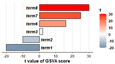
特点: 左右双向条形图。
# 模拟输入数据 GSVA的输出结果,包含name和t两列
rs1=data.frame(
  name=c('term1', 'term2', 'term3', 'term4', 'term5', 'term6', 'term7', 'term8'),
  t=c(-20,-10,2,5,15, 16,25,30)
)
head(rs1)


# 绘图函数
drawGSVA=function(data, n=10){
  #n=3 #20
  data_0 = rbind(
    data[order(data$t,decreasing = T),][1:n,], #选择t值最极端的2*n个
    data[order(data$t,decreasing = F),][1:n,])
  # t的最值,用于优化坐标轴,默认注释掉,不用
  #a = round(min(data_0$t));  b = round(max(data_0$t))

  library(ggplot2)
  # 画barplot
  p=ggplot(data_0,aes(x=reorder(name,t),y=t,fill=t))+
    geom_bar(stat = "identity",colour="black",width = 0.78,position = position_dodge(0.7))+
    xlab("")+ylab("t value of GSVA score") +
    # scale_y_continuous(breaks = seq(a,b,(b-a)/6))+
    coord_flip() # 翻转xy轴

  # 主题修饰
  p=p+theme_bw()+
    theme(panel.grid.major.y = element_blank(),panel.grid.minor.y = element_blank(),
          axis.text.y = element_blank(),panel.border = element_blank(),
          axis.ticks.y = element_blank(),axis.line.x = element_line(),
          axis.text.x = element_text(face="bold"),axis.title.x = element_text(face="bold"))
  # 加上文字
  p2=p+geom_text(aes(y=ifelse(t>0,-1,1),label=name), #文字的y坐标。旋转后
                 hjust=ifelse(data_0$t>0,1,0), #按照t值正负,水平调整文字左右对齐
                 fontface=4,size=3.8
                 )+
    scale_fill_gradient2(low="#366488",high="red",mid="white",midpoint = 0,name="t")+
    # ylim(-60,60) + # 设置y轴的范围
    theme(legend.text = element_text(face="bold"),legend.title = element_text(face="bold"),
          # legend.position = c(0.9,0.3),
          legend.direction = "vertical")
  return(p2)
}

# 测试
drawGSVA(rs1, n=3)
目标图片: Nat Commun. 2020 Widespread transcript shortening through alternative polyadenylation in secretory cell differentiation
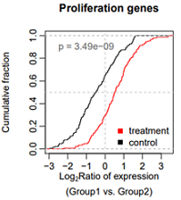
Fig. 4. Single-cell analysis reveals short 3ʹUTRs in SCTs.
(c) Cumulative distribution function (CDF) curves comparing 3ʹUTR APA REDs in SCTs vs. VCTs (from Vento-Tormo et al. data) for genes showing 3ʹUTR shortening in the hESC model (blue curve, 685 genes from Fig. 2c) and all 3ʹUTR APA genes (black curve, 2379 genes). P-value (K–S test) for significance of difference between the two gene sets is indicated.
该图用来比较2个分布的异质性,曲线上升最快的区域对应的x轴区域,是数据集中区域。KS test用于检验2个分布的差异是否显著。
##########
# 累计密度曲线,并做K-S检验
##########
set.seed(2)
control=rnorm(150,-0.5,1)
treatment=rnorm(150, 0.5, 1)
#
hist(control, n=100)
hist(treatment, n=100)
#
pos1=min(c(control, treatment))
pos2=max(c(control, treatment))
## K-S test
rs.test=ks.test(control, treatment)
p=rs.test$p.value;p
p0=formatC(p, format = "e", digits = 2) #保留2位有效数字
p0
# plot
pdf("xx005.pdf", width=3.5, height=4)
plot(ecdf(control), col="black",
     verticals = TRUE, do.points = FALSE, #画竖线,不画点
     cex=0.4, xlim=c(pos1, pos2),
     main="Proliferation genes",
     xlab=expression( atop( paste("Log"["2"], "Ratio of expression"),
                            "(Group1 vs. Group2)") ),
     mgp=c(3,0.6,0),
     ylab="Cumulative fraction")
abline(v=0, col="grey", lty=2)
abline(h=0.5, col="grey", lty=2)

lines(ecdf(treatment), col="red",
      verticals = TRUE, do.points = FALSE,
      cex=0.4)
#添加图例
legend('bottomright',
       box.col = NA, bg = NA,
       legend=c("treatment", "control"),  # text in the legend
       col=c("red","black"),  # point colors
       pch=15)  # specify the point type to be a square
#添加p值
text(-2.5,0.9, adj=0, labels = paste("p", "=", p0), col="#666666")
dev.off()
# Fail: 想把P设置斜体,同时显示P=1.2x10⁻⁹的形式,显示x而不是e,使用上标
#text(-2.5,0.9, adj=0, labels = expression(paste(italic("P"), " =", p0)))
#text(-1.6,0.9,adj=0, labels=p0)
# end
####### density plot with annotation
#########################
# Part I: R base 参考
#########################
set.seed(1)
draws <- rnorm(100)^2
dens <- density(draws)
plot(dens)
q2 <- 2
q65 <- 6.5
qn08 <- -0.8
qn02 <- -0.2
x1 <- min(which(dens$x >= q2))
x2 <- max(which(dens$x < q65))
x3 <- min(which(dens$x >= qn08))
x4 <- max(which(dens$x < qn02))
with(dens, polygon(x=c(x[c(x1,x1:x2,x2)]), y= c(0, y[x1:x2], 0), col="red"))
with(dens, polygon(x=c(x[c(x3,x3:x4,x4)]), y= c(0, y[x3:x4], 0), col="grey"))
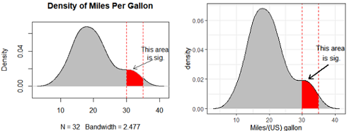
# R base 模仿
d <- density(mtcars$mpg, n=2024) #n越大,后续定位越精细
plot(d, main="Density of Miles Per Gallon",
type="n",ylim=c(-0.01,0.07))
# graphical parameters such as xpd, lend, ljoin and lmitre can be given as arguments.
polygon(d, col="grey", border=NA) # Filled Density Plot
lines(d, col="black") #make outer line clear
# 涂灰色:范围
i1 <- min(which(d$x >= 30));
i2 <- max(which(d$x <= 35))
polygon(x=c( d$x[c(i1, i1:i2, i2)] ), y= c(0, d$y[i1:i2], 0), col="red",
lwd=1, border = "grey")
abline(v=c(30,35), lty=2, col="red")
# 箭头和注释
arrows(x0 = 38, y0 = 0.03, x1 = 32, y1 = 0.02,
# x0, y0,x1,y1 支持一次设置多个值,同时画多个箭头
length=0.1, # length 默认值为0.25, 为了调整不同箭头的大小
code=2, #code : 调整箭头的类型,一共有1,2(默认),3, 共3种类型
#通用的参数,col , lty ,lwd 等
lwd=1, lty=1,
angle=30) #箭头张开角度
text(39,0.038, labels="This area \nis sig.")
#########################
# Part II
#########################
# ggplot2 参考 https://www.jianshu.com/p/c8a886ba5803
#http://www.sthda.com/english/wiki/ggplot2-area-plot-quick-start-guide-r-software-and-data-visualization
# ggplot 模仿
library(ggplot2)
df=data.frame(x=mtcars$mpg)
head(df)
dat <- with(density(df$x), data.frame(x, y))
head(dat)
#
dat1<-dat[dat$x<(30),] #left
dat2<-dat[dat$x>35,] #right
ggplot()+
geom_density(data=df,aes(x=x),fill="red")+
geom_area(data=dat1,aes(x=x,y=y),fill="grey")+
geom_area(data=dat2,aes(x=x,y=y),fill="grey")+
geom_line(data=dat, mapping=aes(x,y), size=0.1, color="black")+ #smooth outer line
geom_vline(xintercept = c(30,35), linetype=2, color="red")+ # vertical line
geom_segment(data = NULL,
aes(x=38,y=0.03, xend=32, yend=0.02), size = 0.8,
arrow = arrow(length = unit(0.3, "cm")))+ #箭头
annotate("text", x =39, y = 0.038, label = "This area \nis sig.") + #文字注释
labs(x="Miles/(US) gallon")+
theme_bw()
两步:1.宽变长,2.画密度分布图。
	> head(apaM.time, 3)
					0h   18h   48h
	chr1:16442:-   102   772   642
	chr1:633932:-   20   123    37
	chr1:944215:- 1277 18445 13133

	> dim(apaM.time)
	[1] 40820     3

# 1.宽变长
pAcounts_per_gene=tidyr::pivot_longer(apaM.time, cols=c("0h", "18h", "48h"),
    names_to ="time",      #变量列名
	values_to ="pAcounts") #值的列名

	> head(pAcounts_per_gene)
	# A tibble: 6 × 2
	  time  pAcounts
	  < chr>    < dbl>
	1 0h         102
	2 18h        772
	3 48h        642

	> dim(pAcounts_per_gene)
	[1] 122460      2


# 2.画图
	> colorset.time
		   0h       18h       48h
	"#FFA500" "#FF1493" "#4876FF"

p2=ggplot(pAcounts_per_gene, aes(x=log10(1+pAcounts), fill=time))+
    geom_density(alpha=0.6)+
    #facet_wrap(~time,
    #    nrow = 3,
    #    scales = "free",
    #)+
    scale_fill_manual(values=colorset.time)+
    theme_classic(base_size = 12)+
    theme(
        #strip.text.x = element_text(angle=0,
        #    #vjust=1,hjust = 1,
        #    size=12), #分面标签 文字倾斜; 字号
        plot.title = element_text(size = rel(1)),
        #strip.background = element_blank()
    )+
    labs(x="lg(pA Counts + 1) per gene", y="Density", fill="time");

pdf( paste0(outputRoot, keyword, "_02_non0-pAreads.time.density.pdf"), width=6, height=2.5)
print(p2)
dev.off()
第一版没有error bar,模仿 fig.3c
ct=c(33, 62, 48, 57)
#
dt2=data.frame(
  length=c("lengthen","lengthen", '', "shorten","shorten"),
  exp=c('up','down', '', 'up','down'),
  #value=c(54,84,NA,85,83)
  value=c(ct[1:2],NA, ct[3:4])
)
dt2

pdf("xx_barPlot.pdf", width=2.8, height=3.8)
par(mgp=c(1.4,0.5,0) )
posX=barplot( rev(dt2$value), col=rev(c("red",'blue','white',"red",'blue')),
              ylim=c(0,70), border=NA, ylab="Gene number" )
text(x=posX, y=rev(dt2$value)+4, labels=rev(dt2$value) )
#text(x=posX-0.3, y=-6, offset = 1,
#     srt = 30, xpd = TRUE, cex=0.9,
#     labels=rev(dt2$exp) )
# arrows
arrows(3.5,-5,6,-5, length = 0.08,
       col='black', xpd = T, code=2, lwd=2)
text(x=5, y=-12,  xpd = TRUE, cex=0.9,
     labels="Lengthen" )
#
arrows(0,-5,2.5,-5, length = 0.08,
       col='black', xpd = T, code=1, lwd=2)
text(x=1, y=-12,  xpd = TRUE, cex=0.9,
     labels="Shorten" )
#
legend(-2.5,-15,xpd = TRUE, horiz=T,
       #box.lwd=3,
       text.width=2.5,
       x.intersp=0.5,
       border=NA, cex=0.8,
       #title="RNA", title.adj=1,
       fill=c('white','blue',"red"), legend = c('RNA level','down', 'up'), bty='n' )
dev.off()
注: 今天发现pdf硬盘占用比png小很多,尝试在网页嵌入pdf图片。缺点是有黑边,不知道怎么去掉。
难点: 对x坐标重排序,对y坐标对数尺度; 组内连线;
library(ggplot2)
library(dplyr)

# 生成数据 ID, treatment, time和values
set.seed(20211103)

mydata = data.frame(
  ID = c(rep(1:10, 2), rep(11:20, 2)),
  treatment = rep(c("v", "p"), each = 20),
  time = rep(c("Before", "After", "Before1", "After1"), each = 10),
  values = c(rnorm(10, mean = 100, sd = 60),
             rnorm(10, mean = 155, sd = 60),
             rnorm(10, mean = 105, sd = 60),
             rnorm(10, mean = 100, sd = 60))
)
mydata$values=10^( mydata$values / ( max(mydata$values)-min(mydata$values) ) *4 )

mydata
summary(mydata$values)
# ID代表受试者的编号;
# treatment有两个水平,v代表疫苗组,p为安慰剂组;
# time分为before和after,分别指代治疗前和治疗后;
# values代表血液中的抗体水平。

str(mydata)
#'data.frame':	40 obs. of  4 variables:
#  $ ID       : int  1 2 3 4 5 6 7 8 9 10 ...
#$ treatment: chr  "v" "v" "v" "v" ...
#$ time     : chr  "Before" "Before" "Before" "Before" ...
#$ values   : num  27.781 21.426 1.857 0.712 9.931 ...

#png("00test.png", width=72*3*0.8, height=72*4*0.8, res=72)
#svg("00test.svg", width=3*0.8, height=4*0.8)
pdf("00test.pdf", width=3*0.8, height=4*0.8, useDingbats=F)
ggplot(mydata, aes(time, log10(values), fill=time))+
  #scale_y_log10()+ #纵坐标取对数
  geom_point(shape=21, size=3, show.legend = F)+
  scale_x_discrete(limits = c("Before", "After", "Before1", "After1"),
                   labels = c("Before", "After", "Before", "After")) +  # 修改x轴刻度上的标签
  scale_y_continuous( breaks = seq(-1,6,1),
    labels = 10^seq(-1,6,1) ) +  # 修改x轴刻度上的标签
  scale_fill_manual(values = c("indianred3", "steelblue", "indianred3", "steelblue")) + # 修改颜色
  geom_hline(yintercept = 2, linetype = "dashed") + # 添加水平虚线
  geom_line(data = filter(mydata, treatment == "v"), aes(group = ID)) + # 添加疫苗组的点对点线条
  geom_line(data = filter(mydata, treatment == "p"), aes(group = ID)) + # 添加安慰剂组的点对点线条
  xlab( "mRNA-xxx    Placebo") +        # 修改x轴的标签
  ylab("Anti-RBD Antibody (U/ml)") + # 修改y轴的标签
  theme_classic()
dev.off()
来源: 群友提问。paper: //todo
后续整理版: 微信公众号 雷达图
喜欢这个GO富集结果可视化效果,距离圆心越远表示越显著,颜色越深表示基因个数越多。
模拟数据文件:
$ cat dustbin/8dat.csv
Desc,id,log10padj,Count
IL-17,1,9.87,11
Rheumatoi,2,7.27,9
Viroal,3,7.16,9
TNF signal,4,5.54,8
Cytokine,5,5.25,11
Chemokine,6,4.98,9
Glycolysis,7,4.69,6
Legionell,8,3.786,5
Lipid and,9,3.782,8
Amoebiasi,10,3.782,6


画图:
# 尝试 v3: 给一个函数版本 //todo
# 两个主要变量:
#  几边形?  10
#  分成几层? 4
#  最大半径? 10


# 多边形数据: 获取圆上的n个点的坐标
# rotate: 为了美观,整体逆时针旋转的弧度
getPointsOnCircle=function( radius=1, npoints=10, center=c(0,0), rotate=pi/2){
  angle=seq(0, 2*pi, length.out=npoints+1)
  xx=center[1] + radius*cos(angle+rotate)
  yy=center[2] + radius*sin(angle+rotate)
  return(data.frame(x=xx, y=yy))
}

# 画多边形
drawPolygon = function(radius, npoints=10, linetype=1, size=0.5){
  geom_polygon(data= getPointsOnCircle(radius, npoints), aes(x, y),
               linetype=linetype,
               size=size, fill="#FFFFFF00", color="#AAAAAA")
}


# (原点到各个顶点)放射线 顶点坐标
getRadialLines = function(maxR=10, npoints=10){
  arr=pi/2 + seq(0, 2*pi, length.out=npoints+1);
  x=c()
  y=c()
  for(i in arr){
    x=c(x, c(0, maxR)*cos(i))
    y=c(y, c(0, maxR)*sin(i))
  }

  return(data.frame(x, y))
}


# 读取数据
dat=read.csv("dustbin/8dat.csv"); head(dat)
dat

# 10个方向上的富集分析: 10边形
dat2=dat
dat2$angle=pi/2+seq(0, 2*pi, length.out=11)[1:10]
dat2$x=dat2$log10padj * cos(dat2$angle)
dat2$y=dat2$log10padj * sin(dat2$angle)
dat2


library(ggplot2)

g1=ggplot()+ xlim(-12, 12) + ylim(-12, 12)+
  drawPolygon(10)+drawPolygon(7.5)+drawPolygon(5)+drawPolygon(2.5)+ #雷达图 几层多边形
  geom_path(data=getRadialLines(10, 10), mapping=aes(x,y), color="#AAAAAA", linetype=1)+ #雷达图放射直线
  geom_polygon(data=dat2, aes(x, y), fill="#CB5656",alpha=0.5, color="#CF0015",size=1 )+ #填充不规则多边形
  #
  geom_point(data=dat2, aes(x,y, fill=Count), size=5, shape=21, color="black", stroke=0.5)+ #添加大点
  scale_fill_gradient(low="white", high="#00B858", breaks=seq(5, 11, 2) )+ #点的渐变色。控制图例数字 breaks+labels
  #
  geom_text(data=data.frame(x=-0.8, y=seq(0,10,2.5) ), aes(x, y, label=y),
            color='black', angle=0, hjust=1, vjust=1 )+ # 仿y坐标值刻度 tick
  annotate(geom="text",x=0.2, y=5,
           label="-log[10]*italic(P)*adj", parse=T,
           color="black", angle=90, vjust=1 )+ #仿y轴名字 label
  #
  geom_text(data=dat2, aes(x=11*cos(angle), y=11*sin(angle), label=Desc), color="black")+# 每条边的文字
  #
  coord_equal()+ #保证x和y轴等长
  theme_void(base_size = 12)+ #去掉坐标轴、边框
  theme(
    legend.position = "top",
    legend.justification = "left", #靠左对齐
    legend.key = element_rect(fill = "black") #不起作用 //todo
  )
g1
pdf("dustbin/radar.pdf", width=4, height=4)
g1
dev.off()
# 输出pdf矢量图,然后可以使用 Illustrator 编辑文字:添加换行、调整文字位置、字号等。
效果图见 边缘密度分布图 | ggExtra包/aplot拼图/ggpubr包 等的实现方法@CSDN
# 1. ggExtra ----
# 1. get data
set.seed(2024)
dat=diamonds[sample(1:nrow(diamonds), 1000),]
library(ggplot2)
# 2. base plot
# with legend
p1=ggplot(dat, aes(carat, price, color=clarity))+
  geom_point()+
  theme_classic()+
  theme(
    panel.border = element_rect(size = 1, colour = "black", fill="#00112200")
  ); p1
# no legend
p2=ggplot(dat, aes(carat, price, color=clarity))+
  geom_point(show.legend = F)+
  theme_classic()+
  theme(
    panel.border = element_rect(size = 1, colour = "black", fill="#00112200")
  ); p2

# 3.margin density
library(ggExtra)
ggExtra::ggMarginal(p1+ggtitle("p1-A"), type = "density")
ggMarginal(p1+ggtitle("p1-B"), colour = "red")

# no legend
ggMarginal(p2+ggtitle("p2-A"), groupColour = TRUE)
ggMarginal(p2+ggtitle("p2-B"),type = "density",groupColour = TRUE,groupFill = TRUE)
ggMarginal(p2+ggtitle("p2-C"),
           xparams=list( fill = c("deeppink")),
           yparams=list( fill = c("navy")),
           color=NA)


## (2) ggExtra::plotCount ----
ggExtra::plotCount(table(scObj$seurat_clusters), fill="orange")+
  theme_classic()+ ggtitle("seurat_clusters")

#dat2=(table(scObj$orig.ident, scObj$seurat_clusters) |> prop.table(margin = 2))*100
#dat2
#ggExtra::plotCount(dat2, fill=c("orange", "darkred" ) )+
#  theme_classic()+ ggtitle("seurat_clusters")

#barplot( (table(scObj$orig.ident, scObj$seurat_clusters) |> prop.table(margin = 2))*100,
#         col=colorset.sample )
#


# 2. ggplot2绘图+aplot拼图 ----
library(RColorBrewer)
len=length( unique(dat$clarity) ); len

# upper density
top_panel <- ggplot()+
  geom_density(data = dat,
               mapping=aes(carat, fill=clarity, color=clarity),
               alpha=0.5)+
  scale_fill_manual(values = brewer.pal(len,'Set2'))+ #设置填充颜色
  scale_color_manual(values = brewer.pal(len,'Set2'))+ # 设置线的颜色
  theme_void()+ # 设置主题
  theme(legend.position="none") # 去除图例
top_panel

# 右侧密度分布图
right_panel <- ggplot()+
  geom_density(data=dat,
               aes(price, fill=clarity,color=clarity),
               alpha=0.5)+
  scale_fill_manual(values = brewer.pal(len,'Set2'))+ #设置填充颜色
  scale_color_manual(values = brewer.pal(len,'Set2'))+ # 设置线的颜色
  theme_void()+ # 设置主题
  coord_flip()+ # 翻转坐标轴
  theme(legend.position="none")# 去除图例
right_panel

# aplot 包拼图
library(aplot)
p1 %>% insert_right(right_panel, width=.4) %>% insert_top(top_panel, height=0.2)
p2 %>% insert_right(right_panel, width=.4) %>% insert_top(top_panel, height=0.2)
#ggsave('plot2.pdf',width = 6,height = 5)


# 3. ggpubr ----
# fig1
library(ggpubr)
gp1<-ggscatterhist(
  iris, x = "Sepal.Length", y = "Sepal.Width",
  color = "Species", size = 3, alpha = 0.6)
gp1
# 不支持theme()
# gp1+theme(panel.background = element_rect(fill="#00112200", color="black"))

# fig2
set.seed(2024)
dat=diamonds[sample(1:nrow(diamonds), 1000),]

ggscatterhist(
  dat, x = "carat", y = "price",
  color = "clarity", size = 2, alpha = 0.6)

# fig3: 指定填充色
ggscatterhist(
  dat, x = "carat", y = "price",
  color = "clarity", size = 3, alpha = 0.6,
  #palette = c("#00AFBB", "#E7B800", "#FC4E07"),
  margin.params = list(fill = "clarity", color = "black", size = 0.2)
)

# Fig4:指定主图黑边框
ggscatterhist(
  dat, x = "carat", y = "price",
  color = "clarity", size = 3, alpha = 0.6,
  #palette = c("#00AFBB", "#E7B800", "#FC4E07"),
  margin.params = list(fill = "clarity", color = "black", size = 0.2),
  ggtheme = theme_classic() + #指定周围边框
    theme(panel.background = element_rect(fill="#00112200", color="black"))
)
欢迎互相切磋,共同进步: 秋秋号 314649593, 请备注大名、来意。
秋秋群: 生物信息与R语言 187923577 禁止营销活动,否则飞机票。
bioToolKit is part of 生物慕课网 www.biomooc.com